- ORI’s lunar descent CTF
Open Research Institute has recently published the solutions for a Lunar Descent CTF that they ran at BSides San Diego 2026. The CTF revolves around the Ka-band radio altimeter used by the Chandrayaan-3 lunar lander. The CTF includes a simulation of the radio altimeter and the goal is to discover why the lander is crashing in this simulation and fix the problem. The CTF is in the Github repository OpenResearchInstitute/lunar-descent-ctf, which includes both the CTF and the solutions (in a
spoilersdirectory). This seemed like an interesting topic, and in the past I have enjoyed a lot other CTFs that were organized by Michelle Thompson, so I decided to clone the repo, delete thespoilersdirectory, and start playing. In this post I comment on the CTF and my solution, so read no further if you don’t want to see spoilers. - Tianwen-2 low data rate telemetry
Thomas Telkamp has shared with me an IQ recording of the Tianwen-2 telemetry downlink made with the Bochum 20 metre antenna on June 8. This is part of an ongoing effort led by Peter Gülzow, AMSAT-DL‘s president, for closely monitoring Tianwen-2’s operations. All the material I have used in previous posts about Tianwen-2 has come from these activities.
This recording was made just before Tianwen-2 did a manoeuvre (recall that the orbital insertion at asteroid Kamo’oalewa was reported to be on June 7). During this recording Tianwen-2 was transmitting telemetry at a slower rate than the usual 16384 baud. This makes sense, given the fact that the attitude during the manoeuvre would be unfavourable. In this short post I decode this recording.
The only two configuration differences between the regular 16 kbaud telemetry and this lower data rate telemetry is that the baudrate is reduced to 4096 baud, and the frame size is reduced to 220 bytes. This means that a single Reed-Solomon codeword from the shortened (252, 220) code is used, instead of four interleaved Reed-Solomon codewords from the full (255, 223) code. The over-the-air frame duration is still one second.
The corresponding modifications to the GNU Radio decoder are simple. This plot shows the decoder running on the recording. The SNR is excellent.
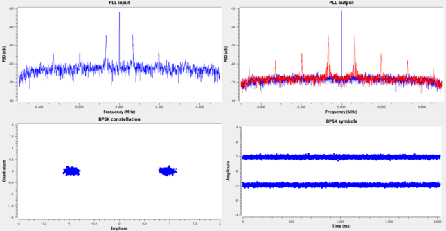
GNU Radio decoder processing the Tianwen-2 low data rate recording The contents of the telemetry frames are the same as the regular 16384 baud telemetry. There are very few differences. One difference is that the last two bytes of the AOS insert zone, which are always
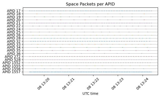
0x300bin 16384 baud telemetry, are always0x0001in this 4096 baud telemetry. I don’t know what these bytes mean, and this difference doesn’t give me a clue either.Almost all the same APIDs as in the regular telemetry are present, although their transmission rate is reduced due to the lower data rate. Comparing, I see that only APIDs 1553 and 1554 are missing in the low rate telemetry.
The GNU Radio decoder used in this post is here, the Jupyter notebook is here, and the binary file containing the decoded frames is here.
- PLL coefficients for rate-only feedback
A couple years ago I wrote a post about the paper Controlled-Root Formulation for Digital Phase-Locked Loops, by Stephens and Thomas. In this paper, the authors study digital PLLs by studying the transfer function in discrete time, rather than doing any continuous-time approximations or equivalences. They give values for the loop coefficients that are needed to achieve a certain noise bandwidth for some standard loop root placements (the supercritical damped response and the standard underdamped response). In general, the loop coefficients are obtained numerically. In my post, I show that in the case of a loop of order 2 with supercritical response the loop coefficients can be calculated explicitly in terms of the loop bandwidth by using the solution of a cubic equation. However, in that post, I treated only the phase/phase-rate feedback case. In this post I cover the rate-only feedback case.
- An update about Tianwen-2 telemetry
Yesterday I posted about my decoding of some recordings of the X-band telemetry of Tianwen-2 done by the Dwingeloo radio telescope. Today I have some small updates.
First of all, I have figured out the format of the AOS insert zone. In the previous post I mentioned that the AOS insert zone contains 8 bytes that are mostly static, except for one byte that seems to be a frame counter. I suspected that the AOS insert zone would contain timestamps, which was the case with Tianwen-1, but this didn’t seem to be the case with Tianwen-2. However, today I have found that the 8-byte insert zone contains a 6-byte timestamp in little endian format that counts the number of \(2^{-16}\) second ticks since the epoch, which is 2019-12-31 16:00:00 UTC (or 2020-01-01 00:00:00 Beijing time). The remaining two bytes have the constant value
0x300b. I don’t know what these two bytes are, since they don’t seem to be a CCSDS time code P-field.There were two things about this timestamp field that were confusing me: the fact that it is little-endian, since CCSDS and the telemetry data in the Space Packet payloads is always big-endian, and the fact that these AOS frames take exactly one second to transmit. This means that the change in the timestamp in each frame is just an increment in the byte corresponding to seconds, which carries over to the next bytes on overflows, plus a very slow drift in the least significant byte caused by the relative drift of the symbol rate clock and the spacecraft clock. Only now that I’ve seen how this field evolves during longer periods of time, I have been able to figure its format.
Using an epoch in Beijing time instead of UTC is common in Chinese spacecraft. For instance, Tianwen-1 uses 2016-01-01 00:00:00 Beijing time as its epoch.
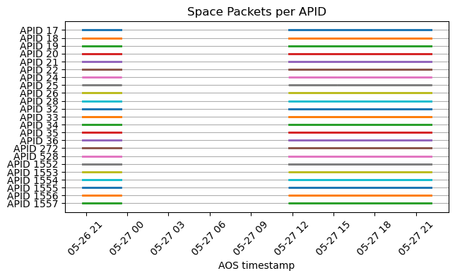
The second update is that AMSAT-DL has been tracking Tianwen-2 with their 20 m dish in Bochum and decoding the telemetry signal in real time with SatDump. They have shared the decoded AOS frames with me, and I have run them through my Jupyter notebook. They have collected a good amount of data: a few hours on May 26 and a full track of about 10 hours on May 27. This data is what has given me the clues to figure out how the timestamps work. The following plot shows the APIDs received over time. This indicates that there are no APIDs that are only active occasionally.
Even though now we have a much longer time span of data, the qualitative behaviour of the telemetry is still the same as I mentioned in the last post. The Jupyter notebook where I analyse the frames received by Bochum is here.
- Decoding Tianwen-2
Tianwen-2 is a Chinese mission that will return samples from the Earth quasi-satellite asteroid 469219 Kamoʻoalewa and rendezvous with the 311P/PanSTARRS comet. It was launched on 28 May 2025 from the Xichang Satellite Launch Center. It is planned to perform its orbital insertion at Kamoʻoalewa on 7 June 2026, and study the asteroid until 24 April 2027. Since ephemerides for this mission are not publicly available, it has been difficult for amateur observers to track it so far, but now it is close enough to Kamoʻoalewa to find it by pointing around the asteroid.
On Monday, CAMRAS used the 25 meter Dwingeloo radio telescope to receive and record the X-band telemetry signal from Tianwen-2, publishing the SigMF recordings in their data archive. They reported that the spacecraft was 1.1 degrees away from the asteroid. In this post I will decode and analyse the telemetry using these recordings.

10ghz artemis1 astronomy astrophotography ATA ccsds ce5 contests digital modes doppler dslwp dsp eshail2 fec freedv frequency gmat gnss gnuradio gomx hermeslite hf jt kits lilacsat limesdr linrad lte microwaves mods moonbounce noise ofdm orbital dynamics outernet polarization radar radioastronomy radiosonde rust satellites sdr signal generators tianwen vhf & uhf