During the last few months, I have been working on gr4-packet-modem. This is a packet-based QPSK modem that I’m writing from scratch using the GNU Radio 4.0 runtime. The gr4-packet-modem project is funded by GNU Radio with an ARDC grant, and its goal is to produce a complete digital communications application in GNU Radio 4.0 that can serve to test how well the new runtime works in this context and also as a set of examples for people getting into GNU Radio 4.0 development. I have presented gr4-packet-modem in the EU GNU Radio days (see the recording in YouTube).
In July, Frank Zeppenfeldt, who works in the satellite communications group in ESA, got in touch with me regarding an opportunity to test gr4-packet-modem on a C-band transponder on Intelsat 37e. His group is running a project with industry about a test campaign of IoT communications over GEO satellites, and they have rented a 1 MHz C-band transponder on Intelsat 37e for some time. The uplink is somewhere around 5.9 GHz, and the downlink somewhere around 3.7 GHz. As part of the project, they have setup a PC and a USRP B200mini in a teleport in Germany that has a large antenna to receive the downlink. There is remote access to this PC, so all the downlink part of the experiments is taken care of: IQ recordings can be made and receiver software can be run in this PC. Therefore, if I could set up an uplink station at home in Madrid (which is actually slightly outside the edge of the Europe C-band beam, as it can be seen in this document), then I would be able to run some tests of gr4-packet-modem by running the transmitter in my laptop and the receiver in the remote PC at the teleport.
As I mentioned to Frank when he proposed this experiment, I haven’t implemented an FEC for the payload of the packets in gr4-packet-modem, because I wanted to have full freedom in setting the size of each packet (to test latency with different packet sizes), and a good FEC scheme usually constraints the possible packet sizes (see gr-packet-modem waveform design for more details). Testing a modem that uses uncoded QPSK over a GEO channel is somewhat pointless, but Frank and I agreed that this would be a fun experiment, even if not too interesting from the technical point of view. In the rest of the post I explain the test set up and results.
DME (distance measuring equipment) is an aircraft radio navigation system that is used to measure the distance between an aircraft and a DME station on ground. DME is often colocated with a VOR station, in which case the VOR provides the bearing information. DME works by measuring the two-way time of flight of pulse pairs, which are first transmitted by the aircraft, then retransmitted with a fixed delay by the ground station, which acts as a transponder, and finally received back by the aircraft. DME operates between 960 and 1215 MHz. It is channelized in steps of 1 MHz, and the air-to-ground and ground-to-air frequencies always differ by 63 MHz (here is a list of all the frequency channels).
I want to write a post explaining in detail how DME works by analysing a recording of DME that contains both the air-to-ground and the ground-to-air channels. Among other things, I want to show that the delay between the aircraft and ground station pulses matches the one calculated using the aircraft position (which I can get from ADS-B data on the internet), the ground station position, the position of the recorder, and the fixed delay applied by the ground station transponder.
Recording two channels 63 MHz apart is tricky with the kind of SDRs I have. Devices based on the AD9361 technically support a maximum sample rate of 61.44 Msps (although some people are running it at up to 122.88 Msps). The LMS7002M, which is used by the LimeSDR and other SDRs, is an interesting alternative, for two reasons. First, it supports more than 61.44 Msps. However, it isn’t clear what is the maximum sample rate supported by the LimeSDR. Some sources, including the LimeSDR webpage mention 61.44 MHz bandwidth, but the LMS7002M datasheet says that the maximum RF modulation bandwidth (whatever that means) through the digital interface in SISO mode is 96 MHz. In the case of the LimeSDR there is also the limitation of the USB3 data rate, but this should not be a problem if we use only 1 RX channel. I haven’t found clear information about the limitations of each of the components of the LMS7002M (ADC max sample rate, etc.).
The second interesting feature is that the LMS7002M has a DDC on the chip. The AD9361 has a series of decimating filters to reduce the ADC sample rate and deliver a lower sample rate through the digital interface. The LMS7002M, in addition to this, has an NCO and digital mixer that can be be used to apply a frequency shift to the ADC IQ signal before decimation.
I had two different ideas about how to use the LimeSDR to record the two DME channels. The first idea consisted in using a 70 Msps output sample rate. For this I used an ADC sample rate of 140 Msps, because I think it is necessary to have at least decimation by 2 after the ADC (the LMS7200M documentation does not explain this clearly, so figuring out how to use the chip often involves some trial and error using LimeSuiteGUI). This idea had two problems. The first problem is that some CGEN PLL occasionally failed to lock when using an ADC sample rate of 140 Msps. However the LimeSuite driver retried multiple times until the PLL locked, so in practice this wasn’t a problem. This approach worked well on my desktop PC, since in 70 Msps I had the two DME channels and then I could use GNU Radio to extract each of the two channels (for instance with the Frequency Xlating FIR Filter). However, the laptop I planned to use to record on the field couldn’t keep up with 70 Msps.
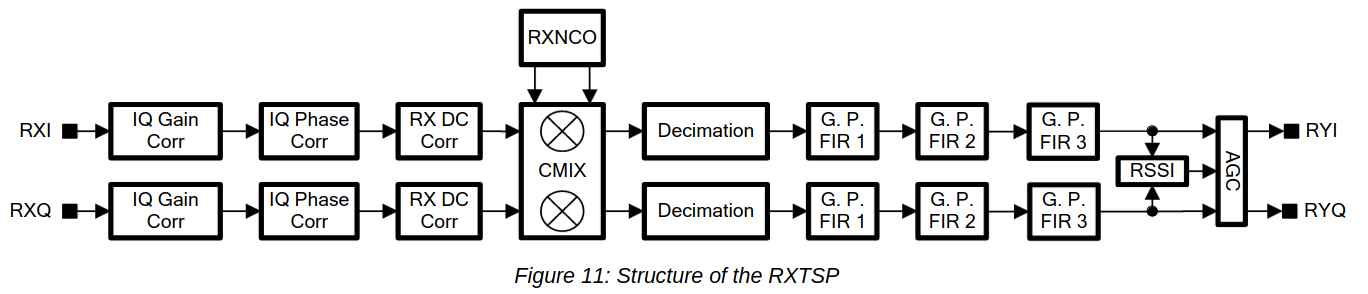
The second idea was to use the on-chip DDC in the LMS7200M to extract the DME channel and deliver a much lower sample rate over the digital interface. The figure below shows how the LMS7200M digital signal processing datapath works. This datapath is called RXTSP. The RXI and RXQ signals are the digital signals coming from the ADC (here and below, by ADC I mean a dual-channel ADC, since the LMS7002M is a zero-if IQ transceiver). The RYI and RYQ are the signals delivered to the digital interface of the chip. Since the LMS7200M has two RX channels, there are two identical chains, one for each channel. The parameters of each chain can be programmed completely independently.
LMS7200M digital signal processing, extracted from the datasheet
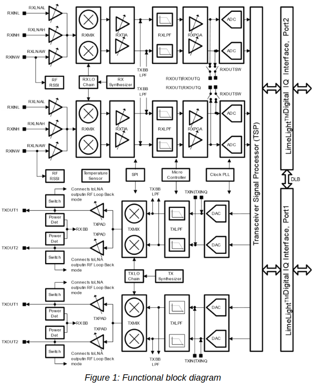
There is no way of sending the signal of one ADC to the two RXTSPs. The connection between each ADC and its corresponding RXTSP is fixed. Therefore, we need to feed in the antenna signal through the two RX channels, but we can easily do this with an external splitter. Remember that both of the LMS7200M RX channels share the same LO, as illustrated by the block diagram below. So the point here is to tune the LO to a frequency between the two DME channels, set the sample rate high enough that both DME channels are present in the ADC output, and finally to use each of the two RXTSPs to extract one of the DME channels, sending it at a low sample rate through the digital interface.
LMS7200M block diagram, extracted from the datasheet
This approach has worked quite well. I have set the ADC to 80 Msps and used the RXTSPs to dowconvert and decimate the DME channels to 2.5 Msps, recording that data directly in GNU Radio.
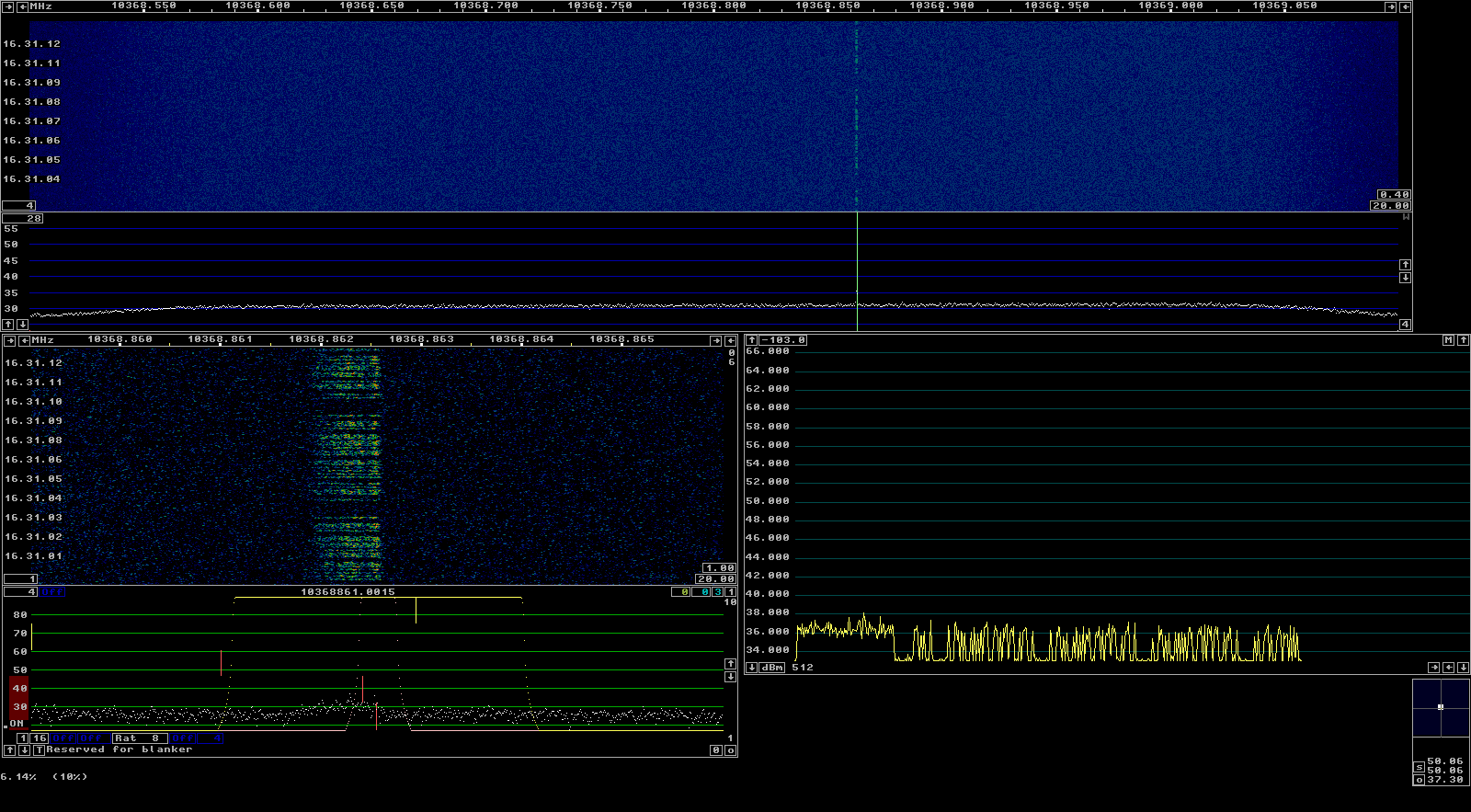
At the beginning of August I visited the Allen Telescope Array (ATA) for the Breakthrough Listen REU program field trip (I have been collaborating with the REU program for the past few years). One of the things I did during my visit was to use an ADALM Pluto running Maia SDR to do a very quick scan of the radio frequency interference (RFI) on-site. This was not intended as a proper study of any sort (for that we already have the Hat Creek Radio Observatory National Dynamic Radio Zone project), but rather as a spoor-of-the-moment proof of concept.
The idea was to use equipment I had in my backpack (the Pluto, a small antenna, my phone and a USB cable), step just outside the main office, scroll quickly through the spectrum from 70 MHz to 6 GHz, stop when I saw any signals (hopefully not too many, since Hat Creek Radio Observatory is supposed to be a relatively quiet radio location), and make a SigMF recording of each of the signals I found. It took me about 15 minutes to do this, and I made 6 recordings in the process. A considerable amount of time was spent downloading the recordings to my phone, which takes about one minute per recording (since recordings are stored on the Pluto DDR, only one recording can be stored on the Pluto at a time, and it must be downloaded to the phone before making a new recording).
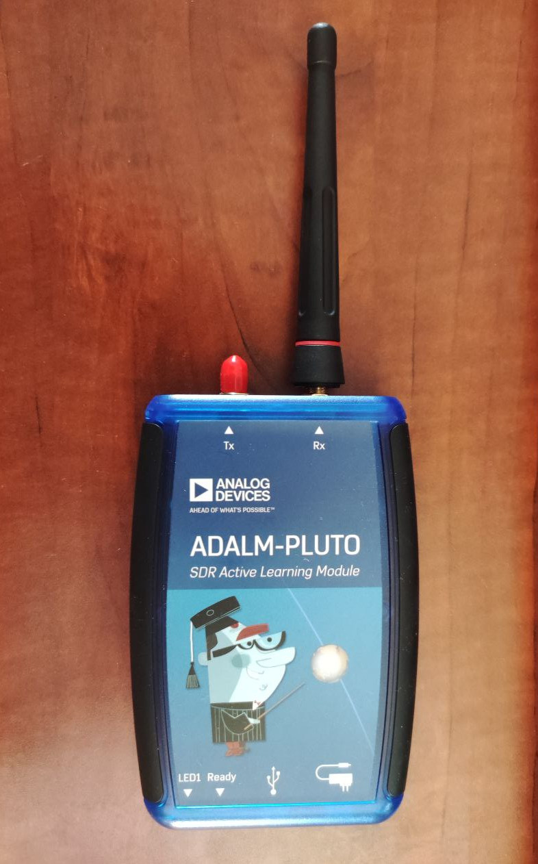
This shows that Maia SDR can be a very effective tool to get a quick idea of how the local RF environment looks like, and also to hunt for local RFI in the field, since it is quite easy to carry around a Pluto and a phone. The antenna I used was far from ideal: a short monopole for ~450 MHz, shown in the picture below. This does a fine job at receiving strong signals regardless of frequency, but its sensitivity is probably very poor outside of its intended frequency range.
ADALM Pluto and 450 MHz antenna
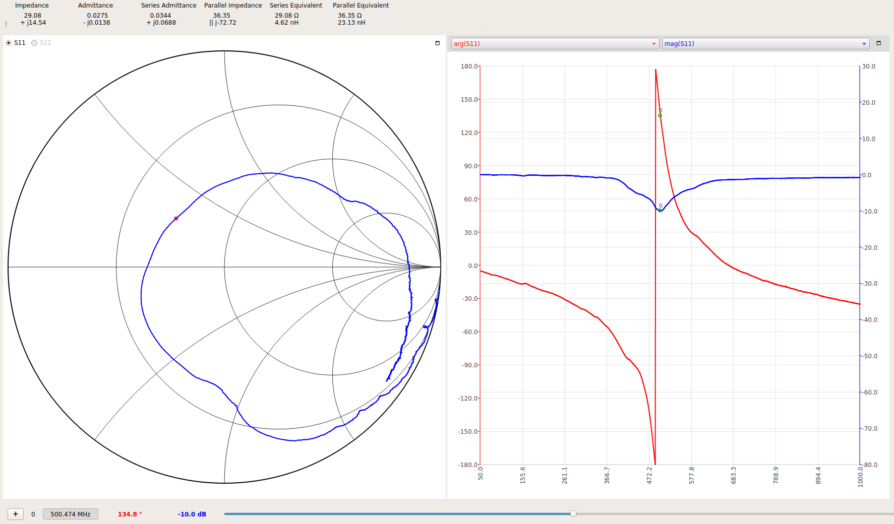
The following plot shows the impedance of the antenna measured with a NanoVNA V2. The impedance changes noticeably if I put my hand on the NanoVNA, with the resonant peak shifting down in frequency by 50 to 100 MHz. Therefore, this measurement should be taken just as a rough ballpark of how the antenna looks like on the Pluto, which I was holding with my hand.
Impedance of the 450 MHz antenna
As the antenna I used for this survey is pretty bad, the scan will only show signals that are actually very strong on the ATA dishes. The log-periodic feeds on the ATA dishes tend to pick up signals that do not bounce off the dish reflectors, and instead arrive to the feed directly from a side. This is different from a waveguide type feed, in which signals need to enter through the waveguide opening. Therefore, besides having the main lobe corresponding to a 6.1 m reflector, the dishes also have relatively strong sidelobes in many directions, with a gain roughly comparable to an omnidirectional antenna. The system noise temperature of the dishes is around 100 to 150 K (including atmospheric noise and spillover), while the noise figure of the Pluto is probably around 5 dB. This all means that the dishes are more sensitive to detect signals from any direction that the set up I was using. In fact, signals from GNSS satellites from all directions can easily be seen with the dishes several dB above the noise floor, but not with this antenna and the Pluto.
Additionally, the scan only shows signals that are present all or most of the time, or that I just happened to come across by chance. This quick survey hasn’t turned up any new RFI signals. All the signals I found are signals we already knew about and have previously encountered with the dishes. Still, it gives a good indication of what are the strongest sources of RFI on-site. Something else to keep in mind is that the frequency range of the Allen Telescope Array is usually taken as 1 – 12 GHz. Although the feeds probably work with some reduced performance somewhat below 1 GHz, observations are done above 1 GHz. Therefore, none of the signals I have detected below 1 GHz are particularly important for the telescope observations, since they are not strong enough to cause out-of-band interference.
I have published the SigMF recordings in the Zenodo dataset Quick RFI Survey at the Allen Telescope Array. All the recordings have a sample rate of 61.44 Msps, since this is what I was using to view the largest possible amount of spectrum at the same time, and a duration of 2.274 seconds, which is what fits in 400 MiB of the Pluto DDR when recording at 61.44 Msps 12 bit IQ (this is the maximum recording size for Maia SDR). The published files are as produced by Maia SDR. At some point it could be interesting to add additional metadata and annotations.
In the following, I do a quick description of each of the 6 recordings I made.
W-Cube is a cubesat project from ESA with the goal of studying propagation in the W-band for satellite communications (71-76 GHz downlink, 81-86 GHz downlink). Current ITU propagation channel models for satellite communications only go as high as 30-40 GHz. W-Cube carries a 75 GHz CW beacon that is being used to make measurements to derive new propagation models. The prime contractor is Joanneum Research, in Graz (Austria). Currently, the 75 GHz beacon is active only when the satellite is above 10 degrees elevation in Graz.
Some months ago, a team from ESA led by Václav Valenta have started to make observations of this 75 GHz beacon using a portable groundstation in ESTEC (Neatherlands). The groundstation design is open source and the ESA team is quite open about this project. I have recently started to collaborate with them regarding opportunities to engage with the amateur radio community in this and future W-band propagation projects (there is an amateur radio 4 mm band, which usually covers from 75.5 to 81.5 GHz, depending on the country). As I write this, some of my friends in the Spain and Portugal microwave group are running tests with their equipment to try to receive the beacon.
On 2023-06-16, the team made an IQ recording of the beacon using their portable groundstation. They have published some plots about this observation. Now they have shared the recording with me so that I can analyse it. One of the things they are interested in is to evaluate the usage of the gr-satellites Doppler correction block to perform real-time Doppler correction with a TLE. So far they are doing Doppler correction in post-processing, but due to the high Doppler drift, it is not easy to see the uncorrected signal in a spectrum plot.
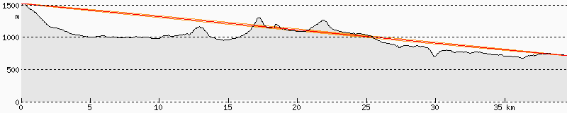
Yesterday we had a strong storm in Madrid at around 16:30 UTC. The storm was rather short but intense. Seeing the heavy rain, it occurred to me that I might be able to receive the 10 GHz beacon ED4YAE at Alto del León using my QO-100 groundstation (without moving the antenna).
The 10 GHz beacon is 39.4 km away and the direct path to my station is obstructed by some hill in the middle, as shown in the link profile.
In the countryside just outside town it is possible to receive the beacon, probably because it diffracts on the hills. However, it is impossible for me to receive it directly from home, as there are too many tall buildings in the way.
In fact, when I fired up my receiver as the storm raged, I was able to see the beacon signal, with a huge Doppler spread of some 700 Hz (20 m/s). The CW ID of the beacon was easy to copy.
ED4YAE -> EA4GPZ at 10 GHz via rain backscatter
Then I started recording the signal. As the rain got weaker, it started disappearing, until it faded away completely. This post is a short analysis of the scatter geometry and the recording.
Back in 2019, I took advantage of the autumn sun outage season of Es’hail 2 to make some observations as the sun passed in front of the fixed 1.2 metre offset dish I have to receive the QO-100 transponders. Using the data from those observations, I estimated the gain of the dish and the system noise. A few weeks ago, I have repeated this kind of measurements in the spring sun outage season this year. This post is a summary of the results.
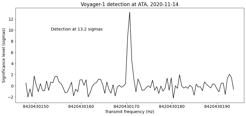
This post has been delayed by several months, as some other things (like Chang’e 5) kept getting in the way. As part of the GNU Radio activities in Allen Telescope Array, on 14 November 2020 we tried to detect the X-band signal of Voyager-1, which at that time was at a distance of 151.72 au (22697 millions of km) from Earth. After analysing the recorded IQ data to carefully correct for Doppler and stack up all the signal power, I published in Twitter the news that the signal could clearly be seen in some of the recordings.
Since then, I have been intending to write a post explaining in detail the signal processing and publishing the recorded data. I must add that detecting Voyager-1 with ATA was a significant feat. Since November, we have attempted to detect Voyager-1 again on another occasion, using the same signal processing pipeline, without any luck. Since in the optimal conditions the signal is already very weak, it has to be ensured that all the equipment is working properly. Problems are difficult to debug, because any issue will typically impede successful detection, without giving an indication of what went wrong.
I have published the IQ recordings of this observation in the following datasets in Zenodo:
AMICal Sat was finally launched on 2020-09-03, and since them the satellite team has been busy trying to downlink some images, both using the UHF transmitter (which uses the same protocol as Światowid) and the S-band transmitter. This has proven a bit difficult because the ADCS of the satellite is not working, and the downlink protocols are not very robust.
Julien has been sending me recordings done by their groundstation in Russia with the hope that we could be able to decode some of the data. Before several failed attempts where we were hardly able to decode a few packets, we got a particularly good S-band recording done on 2020-10-05. Using that recording, I have been able to decode a full image.
In a previous post I talked about how the high data rate signal of Tianwen-1 can be used to replay recorded telemetry. I did an analysis of the telemetry transmitted over the high speed data signal on 2020-07-30 and showed how to interpret the ADCS data, but left the detailed description of the modulation and coding for a future post.
Here I will talk about the modulation and coding, and how the signal switches from the ordinary low rate telemetry to the high speed signal. I also give GNU Radio decoder flowgraphs, tianwen1_hsd.grc, which works with the 8192 bit frames, and tianwen1_hsd_shortframes.grc, which works with the 2048 bit short frames.