Sun observations at 10GHz

Around October 9 it was the sun outage season for Es’hail 2 as seen from Madrid. This means that the sun passed behind Es’hail 2, so it was the perfect occasion to observe the sun with my QO-100 groundstation, which has a 1.2m offset dish antenna pointing to Es’hail 2. This is an account of the measurements I made, and their use to evaluate the receiver performance.

To measure the noise power I used a LimeNET Micro with the following GNU Radio companion flowgraph, which computes and stores to disk average power readings every second. An observation frequency of 10488MHz and a bandwidth of 5MHz were used. It was noted that with a higher bandwidth the LimeNET Micro lost samples. The LNB used was an Avenger PLL321S-2 modified to use an external 27MHz reference, which was supplied from a GPSDO. The LimeNET Micro was disciplined using its onboard GPS. The recording was analyzed in this Jupyter notebook.

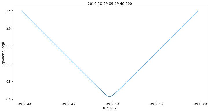
According to the NORAD TLEs, Es’hail 2 was located at an azimuth of 138.92º and elevation of 34.23º as seen from my station. It is assumed that the dish was aimed close to this location, but still we keep in mind a possible pointing error. The figure below shows the separation between the sun and Es’hail 2 on October 9, which was the day of closest separation. The time of closest separation was 09:49:40 UTC. On other days around October 9, the sun also passed nearby Es’hail 2 at around 09:50 UTC, but not so near as on October 9.

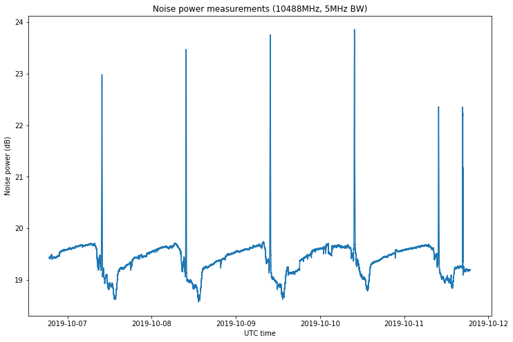
The figure below shows the noise measurements recorded over the course of five days. We see the noise spike up at around 09:50 UTC each day when the sun passes through the beam of the dish. The second spike on October 11 is a Y-factor measurement that will be described later. We observe that the noise changes in a daily pattern due to the LNB gain changing with temperature. We have more noise at night when the LNB is cooler.

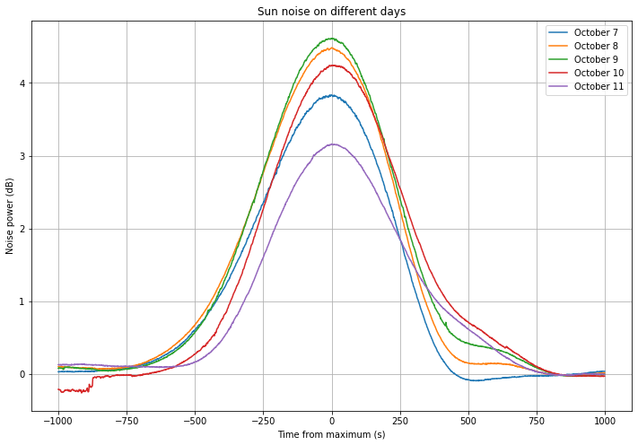
Below we show the observation of the sun noise on each of the five days as the sun passes through the beam of the dish. They observations show sun noise plus “sky” noise (defined as the antenna temperature plus the receiver noise) and they have been scaled to show the sky noise as 0dB. The observations have been arranged so that the maximum is attained at the middle of the graph. The maximum noise obtained is 4.6dB.

In the figure below we show the location of the sun corresponding to each of the curves in the figure above. The colour coding is the same, so the blue curve corresponds to October 7 and the purple curve corresponds to October 11. The point on each curve where the noise attained its maximum value is shown with a black dot, and the location of Es’hail 2 is shown with a red cross.

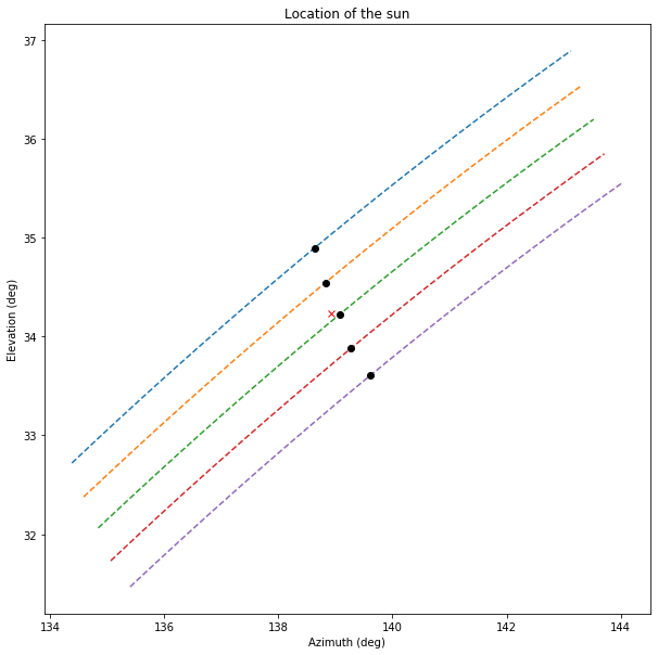
Since the days where more noise was measured are October 8 and 9, which showed similar noise values, this means that the location of the dish pointing was approximately halfway between the black dots on the yellow and green curves. This is close to the nominal location of Es’hail 2. The angular separation between the dots on the yellow and green curves is 0.38º. Therefore, an educated guess for the angular distance between the dot on the green curve and the dish pointing is 0.15º.

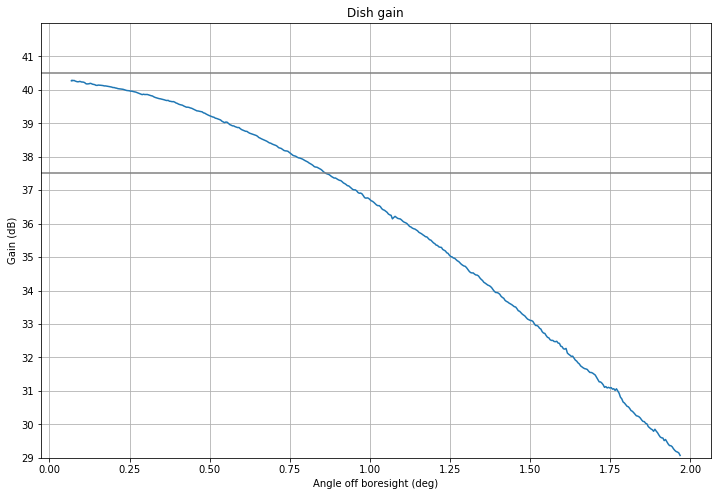
Next, the dish gain is calculated by using the method I described in this post with the sun noise measured on October 9. A gain of 40.5dBi is obtained, with a 3dB half-beamwidth of 0.85º, and a 10dB half-beamwidth of 1.8º. The measured antenna pattern is shown below.

Now we turn to the evaluation of the receiver performance. First we will compute the expected sun noise power at the receiver. The Learmonth observatory gave the following values for the solar radio flux on October 9.

IFLUX : Background Solar Radio Flux
-----------------------------------
Station Date Time Status Freq QS flux Quality
Learmonth 09/10/19 03:24 final 245 13 good
410 26 good
610 34 good
1415 45 ?
2695 66 good
4995 106 good
8800 228 good
15400 554 good

Interpolated value for 1300MHz: 43.7
Interpolated value for 1540MHz: 47.3
Interpolated value for 1707MHz: 50.3
Interpolated value for 2300MHz: 60.1
Interpolated value for 2401MHz: 61.6
Interpolated value for 2790MHz: 67.8
Interpolated value for 5625MHz: 124.5
Interpolated value for 6000MHz: 135.8
Interpolated value for 8000MHz: 200.4
Interpolated value for 8200MHz: 207.2
Interpolated value for 9410MHz: 253.6
Interpolated value for 10400MHz: 297.2

Thus, we take as 297.2Jy the solar flux at the observing frequency of 10488MHz.

The aperture \(A\) of the receiving antenna can be computed in terms of its gain as\[A = \frac{G\lambda^2}{4\pi},\]where \(G\) is the gain and \(\lambda\) is the wavelength. With the gain of 40.5dBi we have measured above, we obtain an aperture of 0.73\(\mathrm{m}^2\).

The efficiency of the dish is defined as the aperture divided by the physical dish collecting area. We can give a rough estimate for the collecting area by assuming that the dish seen from boresight looks as a circle of radius \(r = 0.6\mathrm{m}\), so its area is \(\pi r^2\). Using this estimate for the area we obtain an efficiency of 0.65, which is typical for an offset dish.

The power spectral density of the sun noise received at the LNB probe can be computed as\[P=\frac{1}{2}\gamma FA,\]where \(F\) denotes the radio flux in \(\mathrm{W}/(\mathrm{m}^2·\mathrm{Hz})\), and \(\gamma\) is a dimensionless quantity that accounts for losses, to be described later. The factor 1/2 accounts for the fact that the probe only receives one polarization, while the radio flux is unpolarized.

We now break up the parameter \(\gamma\) into the different losses that are present in the system. First, we have the atmospheric losses \(\gamma_a\). A simple model is given in this article:\[\gamma_a = \gamma_{a,z}^{\frac{1}{\sin \varepsilon}},\]where \(\gamma_{a,z}\) denotes the zenith attenuation, which has a typical value of -0.22dB at 10GHz and \(\varepsilon\) is the elevation. For an elevation of 34.23º we obtain \(\gamma_a = -0.39\mathrm{dB}\).

Next, we have losses \(\gamma_c\) due to the plastic dust cover of the LNB. These are estimated in the article as -0.1dB. Another loss we need to consider is the losses \(\gamma_p\) due to pointing error. For the pointing error of 0.15º we have estimated above, the antenna gain has been reduced by some 0.4dB, so we set \(\gamma_p = -0.4\mathrm{dB}\).

Finally, this other article gives a beamsize correction that should be used when the sun occupies a considerable portion of the antenna beam. The correction can be modeled as the loss factor\[\gamma_b = (1+0.38(w_s/w_a)^2)^{-1},\]where \(w_s\) is the diameter of the radio sun, which is 0.5º for frequencies above 3GHz, and \(w_a\) is the antenna 3dB beamwidth, which is 1.7º in our case. Thus, we obtain \(\gamma_b = -0.14\mathrm{dB}\).

Therefore the total losses are \(\gamma = \gamma_a \gamma_c \gamma_p \gamma_b = -1.03\mathrm{dB}\).

Using the formula above, we obtain a power spectral density of \(8.55\cdot 10^{-21}\mathrm{W}/\mathrm{Hz}\). This can be expressed as a noise temperature in K by dividing by Boltzmann’s constant \(k_B\), obtaining 619K.

Now we compare the sun and “sky” noise (defined as the noise received when the sun is not present in the beam). We interpret these in terms of signal to noise ratios, with the sun noise being the signal and the sky noise being the noise. We have obtained a signal plus noise to noise ratio of 4.6dB. This gives a signal to noise ratio of 2.77dB. Dividing the sun noise by this signal to noise ratio, we obtain a sky noise of 327K.

Let us now study whether this value of 327K for the sky noise is reasonable. On October 11, a Y factor measurement was made where the LNB was pointed to the (hot) ground and the noise power was compared with the (cold) sky noise. A Y factor, or difference, of 2.9dB was measured between the hot and cold temperatures. The ambient temperature was 21ºC, so the hot temperature was \(T_h = 294\mathrm{K}\). The Y factor relates the hot temperature \(T_h\) and the cold temperature \(T_c\), which is mainly due to dish spillover (it also includes the cosmic microwave background) by\[T_h + T_s = Y(T_c + T_s),\]where \(T_s\) denotes the system noise temperature, which is dominated by the LNB noise temperature. The sky noise we have determined above is simply \(T_c + T_s\).

Now, obtaining a good estimate of \(T_c\) is difficult, since the spillover depends greatly on how well the dish is illuminated. In a previous post I had used an estimate of 70K for the spillover, which was taken from the experiments by Ian Roberts ZS6BTE. However, if we accept as valid the sky noise value of \(T_c + T_s = 327\mathrm{K}\) given above, we can solve for the system noise as \(T_s = Y(T_c + T_s) – T_h = 346\mathrm{K}\). This is impossible, since it would imply \(327\mathrm{K} = T_s + T_c > T_s = 346\mathrm{K}\).

This means two things. First, that we have understimated somewhat the losses when computing the power spectral density of the sun noise. As an example, with an additional -0.5dB of losses we would get a sky noise of 292K, which gives a system noise of 276K and a cold temperature of 15K due to spillover. The second thing is that the spillover can’t possibly be as large as 70K. This would mean that we have greatly understimated the losses. Indeed, if instead of an additional -0.5dB of losses we consider -1.5dB of additional losses, we get a sky noise of 232K, a system noise of 159K and a cold noise of 72K. Thus, it seems more likely that the spillover is around 15K (which is what some other authors consider) rather than 70K.

The system noise temperature of 276K obtained above corresponds to a noise figure of 2.9dB, which seems rather high for an LNB, but it is not so surprising, because the experiments by Ian Roberts show that the noise figure of Ku-band LNBs degrades quickly below approximately 10.6GHz, as they are designed to work from 10.7GHz to 12.75GHz.

There are some additional -0.5dB of losses that should be accounted to explain correctly the results of the sun observation. My impression is that perhaps the gain of the dish is not as high as 40.5dB, and maybe is 0.2 or 0.3dB lower than this. Also, the beamsize correction \(\gamma_b\) is computed for a situation with no pointing error. Note that if we point with an error of 0.15º, one side of the limb of the sun is already at 0.35º off boresight, in comparison to 0.25º for a perfect pointing. If we compare the gain pattern at 0.35º and 0.25º, we see that they differ by 0.3 or 0.4dB, so the beamside correction \(\gamma_b\) should be larger if there is pointing error.