Here I want to show a technique for measuring the gain of a dish that I first learned from an article by Christian Monstein about the Moon’s temperature at a wavelength of 2.77cm. The technique only uses power measurements from an observation of a radio source, at different angles from the boresight. Ideally, the radio source should be strong and point-like. It is also important that the angles at which the power measurements are made are known with good accuracy. This can be achieved either with a good rotator or by letting an astronomical object drift by on a dish that is left stationary.
I will use the Moon noise measurements that I did last month. It is much better to use the Sun instead, which is much stronger. It is also convenient to remark that the Sun and the Moon are not point-like objects, but rather have an apparent radius of around 0.5º. The effects of this will be explained below.
In this post I will be using the notation in the Wikipedia article about antenna gain, where terms such as gain, efficiency and directivity are explained.
When speaking about the gain of a dish, we are really speaking about its directivity. Indeed, if we consider the dish as a transmitting antenna, it is common to assume that all the power radiated by the feed ends up being transmitted somewhere to the far field (even if not in the desired direction). It is reasonable to assume that no power is lost as heat when the radio waves reflect off the dish.
Of course, in a real feed, some power is lost. For instance, Monstein estimates in his article the losses due to the plastic cover in the waveguide of the satellite TV LNB he is using. However, if we are speaking just about the dish itself, it makes sense to assume an lossless feed.
This reasoning justifies that, when considering the gain of a dish, we might take the efficiency of the antenna to be one, so the gain and directivity coincide.
We assume that spherical coordinates \((\theta,\varphi)\) are arranged so that \(\theta \in [0,\pi]\) indicates the angle from the boresight of the dish. Assuming a point-like radio source, the power received when the source is in the direction \((\theta,\varphi)\) is\[P(\theta,\varphi) = \lambda D(\theta,\varphi),\]where \(\lambda\) is a constant and \(D\) denotes the directivity.
By definition of the directivity, we have\[\int_{0}^{2\pi}\int_0^\pi D(\theta,\varphi) \sin \theta\,d\theta d\varphi = \int_{S^2} D(x)\,dA(x) = 4\pi.\]Assuming that the directivity \(D(\theta,\varphi) = D(\theta)\) depends only on \(\theta\), which makes sense, since the radiation pattern of a dish is almost symmetric around the boresight, and that \(D(\theta) = 0\) for \(|\theta| > \theta_0\) for some angle \(\theta_0\), since most of the power radiated by a dish is concentrated in the main lobe of the radiation pattern, then we have\[\int_0^{\theta_0} D(\theta) \sin \theta \, d\theta = 2.\]
This implies that\[\tag{1}\lambda = \frac{1}{2}\int_0^{\theta_0} P(\theta)\sin\theta\,d\theta.\]This integral can be approximated by taking power readings \(P(\theta)\) at different angles from boresight \(\theta\) between 0 and \(\theta_0\). Then the directivity can be computed by dividing the power readings by \(\lambda\), and the gain is simply the directivity in the boresight direction\[G = D(0) = \frac{P(0)}{\lambda}.\]
To perform these calculations, I will use the power readings of Moon noise that I took last month. These can be seen in the graph below.
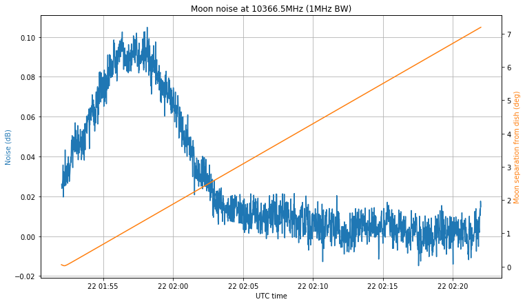
This data has two main problems. First of all, as I commented in my post about the observation, the pointing of the dish was clearly incorrect. The peak of the noise doesn’t happen when the Moon is closest to the nominal dish pointing. Therefore, I have assumed that the Moon passed through the boresight at the moment when the peak in the noise happened, and derived from that the angle from boresight for each of the measurements.
Of course, it is most likely that the Moon didn’t pass exactly through the boresight, but close to it. The effect of this error is to underestimate the gain, though it is not trivial to see this. The calculations will be shown in a future post.
The second problem is that the Moon noise signal is weak. As remarked above, it is best to use a strong signal. The measurements in the figure above are \(S + N\) (signal plus noise). The power measurements used for the computation of the directivity need to consider only the signal power. For very strong signals, \(S + N \approx S\) is a valid approximation. In other cases, we need to come up with an estimate of \(N\) and subtract that from our measurements. For weak signals, the power measurements of \(S\) are very sensitive to the value chosen for \(N\).
When the signal is far enough from the boresight, it is so weak that it is impossible to estimate \(S\) effectively. Thus, \(P(\theta)\) can only be determined with enough accuracy for small \(\theta\), so we need to set the cutoff \(\theta_0\) small enough so that equation (1) only requires measurements \(P(\theta)\) that we are able to make accurately. This has the effect of overestimating the gain, since by choosing \(\theta_0\) too small, we underestimate \(\lambda\).
Nevertheless, the results that can be obtained with my Moon noise measurement are not so bad. The calculations have been done in this Jupyter notebook. The figure below shows the gain or directivity \(D(\theta)\).

The signal power measurements start being too noisy at around 1.6 degrees from boresight, so the cutoff \(\theta_0\) has been put there. We see that the gain of the 1.2m offset dish at 10366.5MHz is approximately 40.5dBi. The 3dB half beamwidth is approximately 1 degree.
The accuracy of this result is not so bad compared with the theory. In this online dish gain calculator, for a 1.2m dish with an efficiency of 0.65 and a frequency of 10366.5MHz, we get a gain of 40.43dBi and a 3dB half beamwidth of 0.81 degrees.
As we have remarked above, the Moon is not a point source. When the radio source is an extended source, then the power measurements are some sort of convolution between the directivity and the power distribution of the source. This has the effect of smearing out the measured antenna pattern, underestimating the gain, and overestimating the beamwidth. The effects are larger when the radio source is large in comparison with the beamwidth.
More in detail, we assume for simplicity that the source is radially symmetric, with a power distribution \(k(\alpha)\), where \(\alpha\) is the angular distance from the centre of the source, normalized so that\[2\pi \int_0^\pi k(\alpha) \sin \alpha \, d\alpha = 1.\]Note that the left hand side of this equality is\[\int_{S^2} k(\alpha(x,y))\,dA(x),\]where \(y \in S^2\) is arbitrary and \(\alpha(x,y)\) denotes the angular distance between the points \(x\) and \(y\).
For example, the Moon or the Sun may be modeled as a uniform disc of angular radius \(\alpha_0\), so that\[k(\alpha) = \frac{1}{2\pi(1-\cos \alpha_0)},\]for \(\alpha \leq \alpha_0\) and \(k(\alpha) = 0\) elsewhere.
Now, the power reading taken at a point \(x \in S^2\) is\[P(x) = \lambda\int_{S^2} D(y) k(\alpha(x,y))\,dA(y).\]Using Fubini’s theorem, we compute\[\begin{split}\int_{S^2}P(x) dA(x) &= \lambda\int_{S^2}\int_{S^2} D(y)k(\alpha(x,y))\,dA(y)dA(x)\\ &= \lambda\int_{S^2} D(y)\,dA(y) = 4\pi\lambda.\end{split}\]Therefore, equation (1) is still a good approximation for \(\lambda\). However, by dividing \(P(x)\) by \(\lambda\), we are computing the convolution\[\int_{S^2} D(y) k(\alpha(x,y))\,dA(y)\]instead of \(D(x)\). Even in the simple case when \(D\) depends only on \(\theta\) and \(k\) describes the uniform disc model given above, the computation of this convolution is rather involved.