On the Beijing time morning of 2020-07-30, Tianwen-1 did something. Paul Marsh M0EYT reports that the probe first switched from the high gain antenna to the low gain antenna, then returned to the high gain antenna, and then switched to a high-speed data mode, finally coming back to the usual 16384baud telemetry.
r00t.cz has already analysed the telemetry data collected during this event. He reports that the high speed data was a replay of the telemetry produced during the period when the low gain antenna was used. He shows some interesting behaviour on APIDs 1280, 1281 and 1282 (see my previous post for a description of these during nominal operation). These seem to contain ADCS data.
This event was followed with some expectation by the Amateur deep space tracking community, since according to this paper Tianwen-1 would make the first correction manoeuvre (TCM-1) early on in the mission (day 9 is stated in the paper). However, by now it is clear that a true correction manoeuvre didn’t happen, since no significant change has been seen in the trajectory described by the state vectors transmitted in the spacecraft’s telemetry. However, this event might have been a very small thruster firing, in order to test the propulsion in preparation for the true TCM-1.
In this post, I look at the data during the high speed replay, following the same approach as in the previous post. With this data, I reach a definite conclusion of what happened during this event (I won’t spoil the mystery by stating it in advance). The description of the modulation and coding used by the high speed data will come in a later post.
The Jupyter notebook for the calculations in this post can be found here.
High speed data
The high speed data is transmitted using 2048kbaud QPSK, and a very similar FEC to the 16368baud ordinary telemetry. Therefore, it is approximately 250 times faster than the ordinary telemetry (the exact calculation should take into account the slight differences in the coding). This means that complete sections of stored telemetry can be replayed very fast.
The high speed data replay done around 2020-07-30 00:45 UTC was only a dozen seconds long, but this was enough to transmit more than 30 minutes of telemetry collected around 2020-07-29 23:40 UTC.
The framing of the high speed data is the same as the ordinary telemetry: AOS frames using M_PDU to store Space Packets. The only difference is that the length of the AOS frames is 892 bytes instead of 220. In this high speed data session only spacecraft ID 245 (which corresponds to the orbiter) was used.
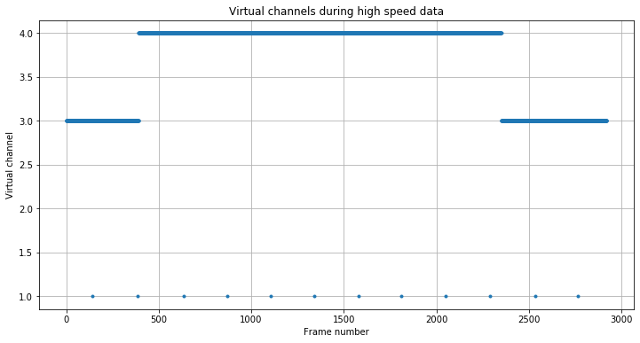
There were three virtual channels used: VC 1, which transmitted only 12 frames and is used to transmit real time telemetry as in the ordinary telemetry, VC 3, which is used to transmit idle frames before and after the transmission of the replay data, and VC 4, which is used to replay recorded telemetry data.
The figure below shows the usage of the different virtual channels during the high speed transmission. We see that virtual channel 1 sends one packet periodically (later we’ll see that it is every second), virtual channel 4 is used in the middle of the transmission, and virtual channel 3 at the beginning and the end.
Virtual channel 1
The frames in virtual channel 1 look the same as those transmitted in the ordinary telemetry. Their timestamps are shown below, where we can see that a frame is transmitted every second. The same APIDs and in roughly the same proportion are sent.
['2020-07-30T00:44:58.880200', '2020-07-30T00:44:59.880200',
 '2020-07-30T00:45:00.888100', '2020-07-30T00:45:01.888400',
 '2020-07-30T00:45:02.884400', '2020-07-30T00:45:03.888300',
 '2020-07-30T00:45:04.884300', '2020-07-30T00:45:05.884200',
 '2020-07-30T00:45:06.884400', '2020-07-30T00:45:07.884300',
 '2020-07-30T00:45:08.884300', '2020-07-30T00:45:09.880200'],
In the ordinary telemetry, a 220 byte frame from virtual channel 1 is sent every 0.5 seconds, because there is a frame every 0.25 seconds, but only 50% of the frames are assigned to spacecraft 245 virtual channel 1. Here, an 892 byte frame is sent every second, so there is plenty of bandwidth to send the same real time telemetry that would be sent with the ordinary telemetry. I haven’t checked if there is a lot of padding in these frames, but if the same telemetry rates are used, there should be approximately 50% of padding in these frames.
Virtual channel 3
The idle frames for virtual channel 3 are similar but not exactly the same as those used in the ordinary telemetry. Most of the frame is filled with 0x55 bytes for padding, instead of 0xaa‘s as in the ordinary telemetry. The only bytes which are not filled with 0x55 are the first 5 bytes of the AOS header and the unknown two byte field in the insert zone, which has the value 0x7aaa.
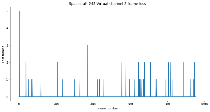
The figure below shows the frame loss for virtual channel 3 (using the virtual channel frame count to detect lost frames). We see that the decoder is working more or less fine, but occasionally we are missing a few frames. The reason will be described in more detail in a future post, but it is mainly due to cycle slips in the Costas loop.
Virtual channel 4
AOS frames from virtual channel 4 have the replay flag in the AOS primary header set to one, indicating that they are used to transmit pre-recorded data rather than real time. The timestamps of these frames are also set in the past and can be used to see what time window is being replayed. This is shown in the figure below.
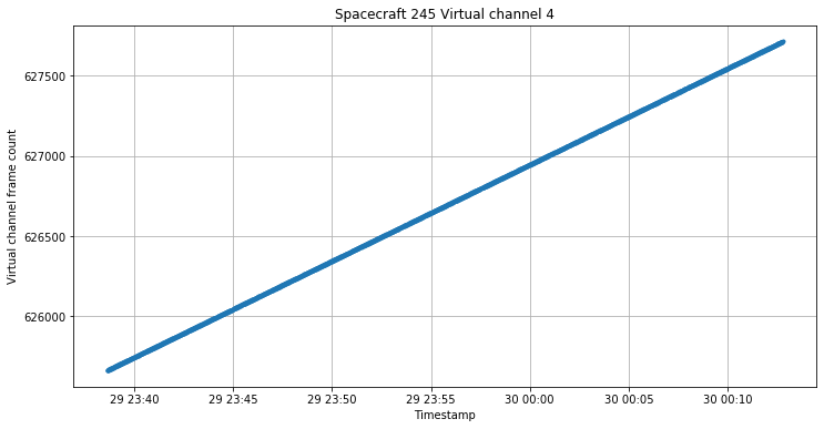
These are the first few timestamps, where we can see that only one frame per (recording) second is sent. As we commented with virtual channel 1, these frames are 4 times as large as those in the ordinary telemetry, so most likely the two 220 byte frames that were sent each second are packed inside a frame and so there is 50% of padding. Or maybe there is extra telemetry that wouldn’t be sent ordinarily. I haven’t checked this.
['2020-07-29T23:38:39.305600', '2020-07-29T23:38:40.305600',
 '2020-07-29T23:38:41.305600', '2020-07-29T23:38:42.305600',
 '2020-07-29T23:38:43.305600', '2020-07-29T23:38:44.305600',
 '2020-07-29T23:38:45.305600', '2020-07-29T23:38:46.305600',
 '2020-07-29T23:38:47.305600', '2020-07-29T23:38:48.305600']
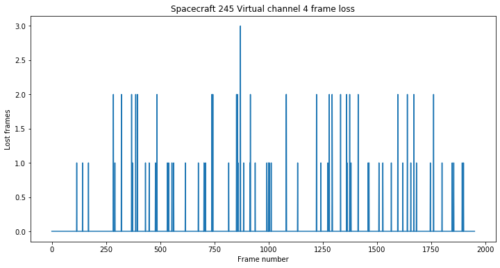
As in the case of virtual channel 3, there is occasional frame loss. Luckily, the number of lost frames is small, so this doesn’t affect our ability to analyse the replayed data.
The APIDs sent in these frames are the same as those sent during the ordinary telemetry on virtual channel 1, and roughly in the same proportions. The value 0x7aaa is sent in the unknown field of the insert zone (this is different from ordinary telemetry).
ADCS data
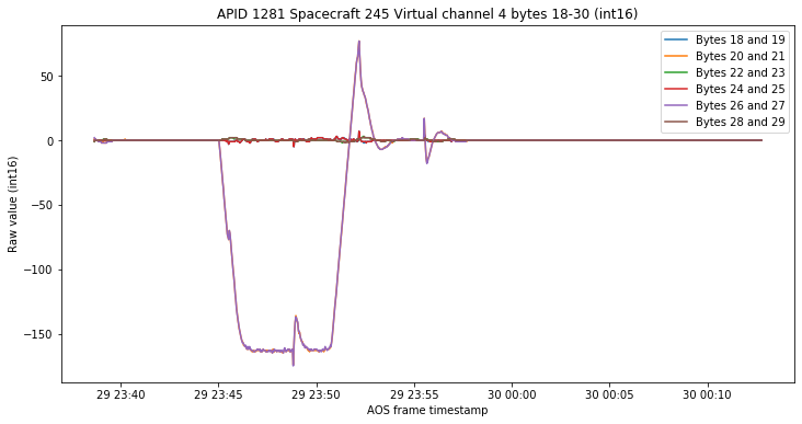
Now we take a look at APIDs 1280, 1281 and 1282, which in the previous post I described as having ADCS data of some sort. During nominal spacecraft coast operations we could see that some channels in these APIDs were zero except for some occasional kicks.
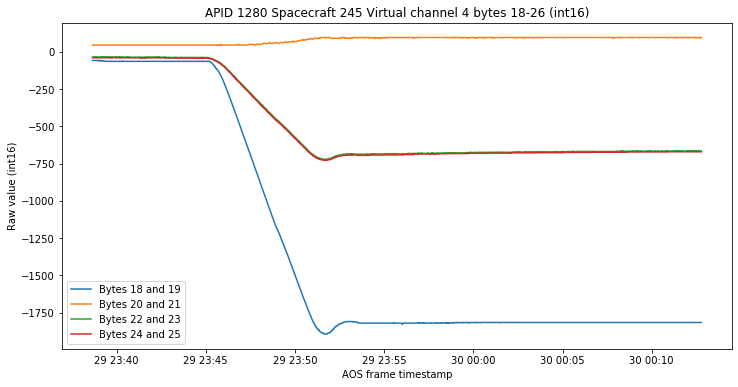
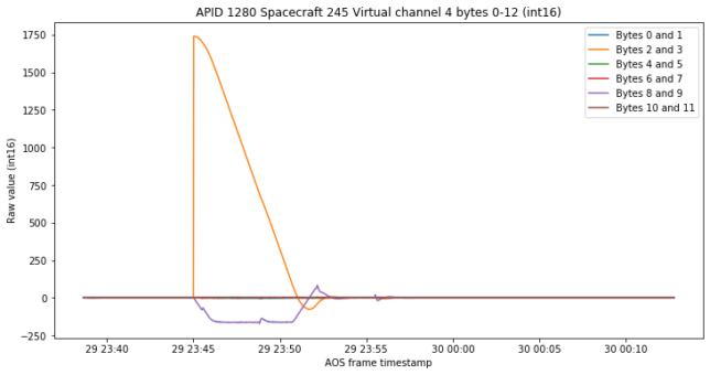
We look at these channels again for the replayed data. The first set of channels is that at the beginning of APID 1280, which I suggested might be the proportional and integral paths of a PI controller. The data we see now reinforces this idea.
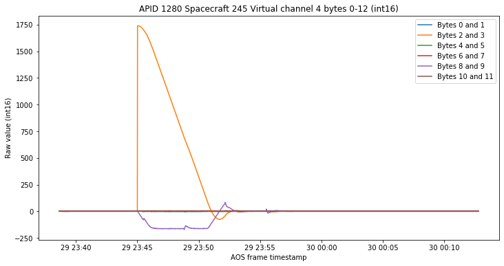
The response is present in the orange and purple channels, which presumably would be the integral and proportional variables corresponding to the second axis (I’ll explain in a more definite way what they are below).
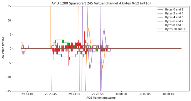
If we zoom in on the vertical axis we see that the response in the other channels is almost inexistent, so everything happens for this second channel.
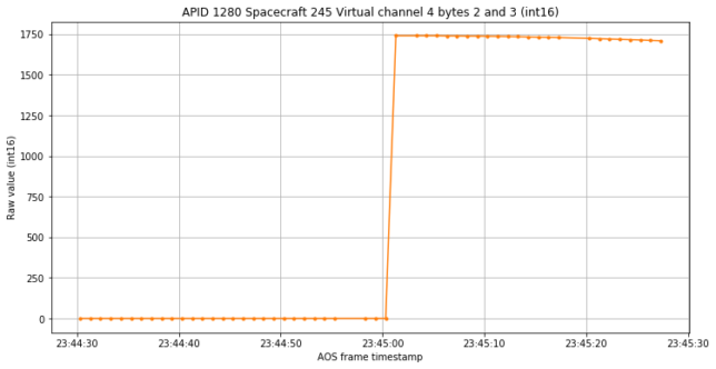
Now, what happens in the orange channel is something non-physical. In fact, zooming in on the time axis we see that the jump from zero to a large value happens instantly. This reinforces the idea that these channels show the state of a controller rather than physical measurements.
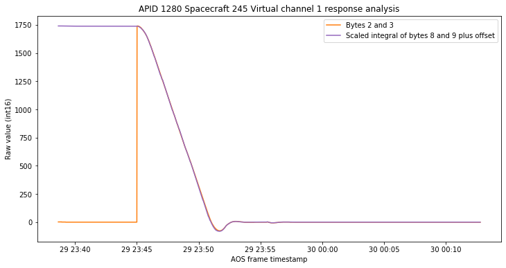
Coming back to the idea that the purple channel is the derivative of the orange channel, we can understand what happens in the following way. This is a PI controller. We want the controller to make some change in the steady state setting. Therefore, we introduce an opposite jump in the integral part (the orange channel) and let the loop compensate for this. The proportional part (purple channel) will start moving in the opposite direction to compensate, thus making the integral part decrease. When both the integral and the proportional part converge again to zero, we have effected a net change in the steady state, since the integral of the proportional part is not zero (basically, it is opposite to the jump we introduced).
To test these ideas, we denote by \(A\) the size of the jump in the orange channel \(O(t)\) and compute and plot\[A – A\frac{\int_{t_0}^t P(s)\,ds}{\int_{t_0}^{t_0+T} P(s)\,ds},\]where \(P(t)\) denotes the purple channel and \(t_0\) and \(t_0+T\) are chosen respectively before and after the whole transient. The results are shown in the figure below. The curve obtained by integration of the purple channel matches very closely the orange channel. This shows that the purple channel is the derivative of the orange channel multiplied by a scale factor.
There are four other channels in APID 1280 that show interesting behaviour. These weren’t shown in my previous post because most likely they had a static value. They are shown below. Three of them seem to have profiles very similar to the integral constructed above from the purple channel, but I’m not so sure about what we’re looking at here.
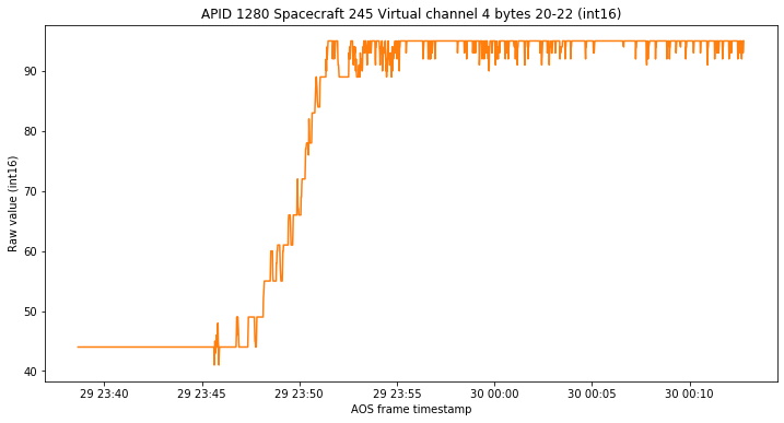
The orange channel deserves being plotted independently, since it is rather noisy and a bit weird.
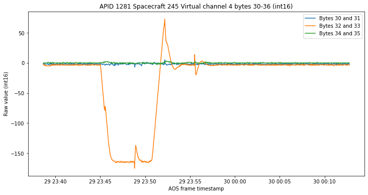
Now we look at the channels from APID 1281 that we studied in the previous post. The first set of channels looks pretty much like the proportional channels from the PI controller, but with some noise. My conclusion is that these are sensors that measure whatever the PI controller is using to compute its error (more details below). There are two sets of 3 channels which have nearly the same values. This can be explained by two sets of redundant sensors.

As in the previous post, the next set of three channels behaves in the same way but is more noisy and the channels have some noticeable bias.
Now we arrive at the key element of this post, which is the following set of four channels. These weren’t studied in the previous post because most likely they had a constant value. These four channels may seem similar to the four channels we’ve plotted for APID 1280 above, but they have a very important property.
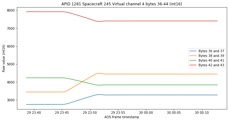
If we interpret these numbers as a 4 dimensional vector and compute its Euclidean norm, we always obtain almost 10000. Here the “almost” is reasonable because of quantization, since the channels’ raw values are integers.
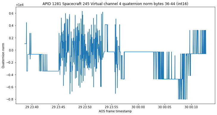
This suggests that these four channels are unit quaternions, with a scale factor of 10000. This scale factor is interesting, since it would perhaps be more natural to use 32767 in order to use the full int16 range, or a power of two (16384 if one doesn’t want to get into trouble with the weird number -32768) to simplify computations. In any case, we interpret these four channels as quaternions encoding the attitude of the spacecraft and see where this leads us.
We denote the quaternion at time \(t\) as \(q(t)\) and by \(t_0\) the start of the replay data and \(t_1\) the end of the replay data. We are not so much interested in the spacecraft orientations themselves but in the change of orientations between \(t_0\) and \(t_1\). Therefore, we consider \(p(t) = q(t) q(t_0)^{-1}\), which describes the relative rotation of the spacecraft from its starting attitude. We have \(p(t_0) = 1\) and then it moves smoothly to the final relative rotation \(p(t_1)\).
Quaternions encode a rotation in three-dimensional space, and (except in degenerate cases) this rotation has an axis, described by a three-dimensional vector, and a rotation angle about this vector. These can be directly computed from quaternion. We compute and plot the vector corresponding to \(p(t)\).

At first, the vector we get is just random, because the rotation is very close to “no rotation” (\(p(t)\) close to 1), so determining the rotation angle is ill-conditioned. However, as the quaternions \(q(t)\) start to change and \(p(t)\) moves away from 1, we get the same rotation vector all the time. This totally makes sense. In principle, these quaternions can describe any rotation following a complicated trajectory, but the simplest way to change the spacecraft’s attitude is to keep rotating about a single constant axis (chosen appropriately) until the desired new attitude is obtained.
The rotation vector is
[-0.14468192, -0.49106965, 0.85902139]
This is expressed in coordinates according to reference frame in which the quaternions are written. It would be interesting to know the reference frame (ICRF perhaps), but for our purposes it is not important, because we prefer to know the rotation axis relative to the spacecraft’s initial orientation.
To do so, we can convert the quaternion \(q(t_0)\) to a rotation matrix. We obtain
[[-0.61269098, -0.14412949,  0.77706914],
 [ 0.72610204, -0.49089391,  0.48145508],
 [ 0.31206664,  0.85921467,  0.40541899]]
The columns of this matrix give the three axes of the spacecraft body in terms of the reference frame. We see that the rotation vector almost coincides with the second column. This means that the axis of rotation is the Y axis of the spacecraft’s body.
Now we compute the rotation angle described by the quaternions \(p(t)\). This is shown below. We see that the spacecraft starts rotating until it achieves a final rotation of -14.99 degrees, with an overshoot of nearly 1 degree.
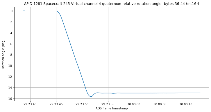
So my conclusion in the light of these quaternions is that what happened during the event described by the replay data is simple: the spacecraft rotated -14.99 degrees about its Y axis. This explains a number of things.
First, the need to switch to the low gain antenna is clear, since the beam of the high gain antenna is going to lose the Earth completely. Second, we can revisit the other channels in APIDs 1280 and 1281 to learn more about them. To do so, it helps to plot the time derivative of the rotation angle.
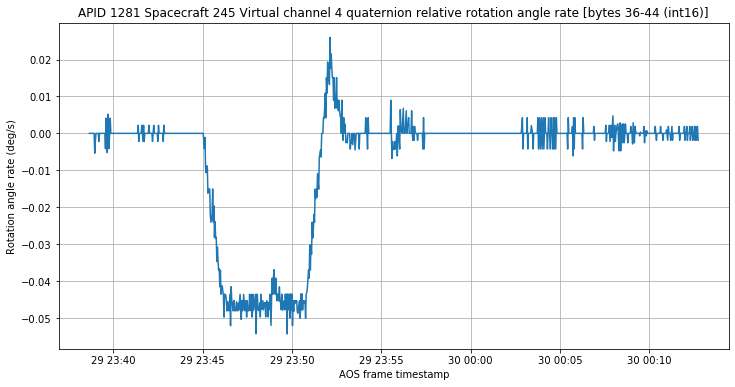
We see that, even though a bit noisy, this has the same shape as many of the channels shown above. This means that those channels correspond to rotation rate, and those which are sensors are most likely gyroscopes.
We come back to the figure with the PI controller data. This is the attitude rotation controller. The purple channel must represent rotation angle rate about the Y axis, and the orange channel is essentially its integral, so it must represent rotation angle about the Y axis.
In more simple terms, the blue, orange and green channels give rotation angle error for the X, Y and Z spacecraft body axes. The error is defined as the current angle minus the desired angle. The red, purple and brown channels give the rotation angle rate error for the X, Y and Z spacecraft body axes. The error is defined as the current angle rate minus the desired angle rate.
In the steady state, both the angle error and the angle rate error are zero. At some point, the system decides to perform a rotation about the Y axis. This changes the desired angle, so the angle error (orange) suddenly jumps and the controller does its thing to drive the angle error and the angle rate error to zero. When it finishes, the desired rotation has been performed. Since this is a rotation about the Y axis, there is virtually nothing in the X and Z channels.
If the data in APID 1281 corresponds to sensors, then these must be gyroscopes, or some other kind of angle rate sensor. There is something quite interesting, which are the kinks in the gyroscope data. These can also be seen in the controller’s angle rate error. We have one small kink as the spacecraft is accelerating its rotation, a large kink when the spacecraft is rotating at a constant angle rate, and another large kink when the spacecraft has come to a stop. This means that there is something preventing the spacecraft from rotating smoothly without glitches.
The other angle rate sensors in APID 1281 are more noisy and have bias, so they might be lower quality gyroscopes. Bias is in fact a problem with low quality gyroscopes.
The scale factors to convert these channels to degrees and degrees per second can be derived from the quaternion data. We know that the total rotation angle is -14.99 degrees, so that sets the scale factor for the angle error channels. We also know that the steady rotation angle rate is around -0.45 degrees per second, so that sets the scale factor for the angle rate error and gyroscope channels.
We now proceed to APID 1282, where there are 7 channels showing interesting behaviour. The patterns are similar to the rotation rate, but not exactly the same. They also have different non-zero values which change between before and after the rotation. The kinks also appear in these channels.
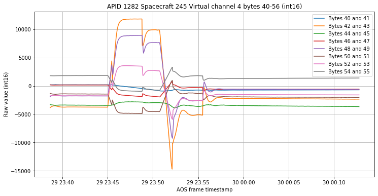
My guess is that these are the flywheels that are effecting the rotation of the spacecraft, but I have haven’t given this idea a serious thought.
Finally, another channel in APID 1282 has interesting data. I have no clue what this is, but it seems to be synchronized to the rotation and the kinks.

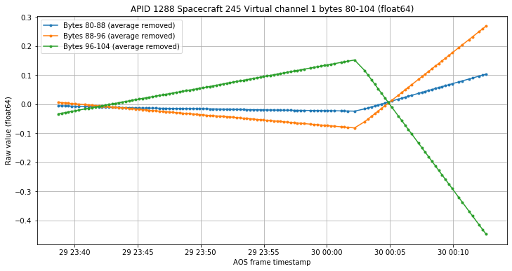
I have also plotted the float64 channels in APID 1288 (see the previous post) to see if they change as a consequence of the rotation.

At first glance these seem static, but if we remove the average of each channel, we see that there are two different linear trends. The change happens a few minutes after the rotation has finished, so I don’t know if the two are connected or this is just a coincidence.
So to summarize, we have seen the spacecraft performing a rotation of -14.99 degrees about the Y axis by studying the telemetry replayed over the high-rate QPSK downlink. While doing so we have gained a better understanding of the ADCS telemetry. Everything seems to indicate that this was just an attitude change manoeuvre.
Now, why was this manoeuvre done? Maybe this was a test for the upcoming TCM-1, which is expected to happen in one of the next few days. It seems that no burn was performed, but maybe a test of the TCM-1 was done by doing everything except for the burn. This would allow checking if the spacecraft is able to change its attitude with the precision needed for the burn.
While not shown in the replay data, it is apparent that the spacecraft returned to the nominal attitude shortly afterwards, since the high gain antenna came back on and the signal was good. This suggests that the satellite team was mostly interested in studying the change from the nominal attitude to the test attitude and only replayed that portion of the data.
7 comments