On 2020-08-01 23:00 UTC, Tianwen-1 made its first correction manoeuvre, called TCM-1. The manoeuvre was observed by Amateur trackers, such as Edgar Kaiser DF2MZ, Paul Marsh M0EYT, and the 20m antenna at Bochum observatory, operated by AMSAT-DL. The news of the successful manoeuvre appeared in Chinese media, and in the German Wikipedia article for Tianwen-1 (thanks to Achim Vollhardt DH2VA for sharing this information).
Since Tianwen-1 transmits its own real time orbit state vectors in the telemetry, by comparing the vectors transmitted before and after TCM-1, and also by studying the Doppler observed by groundstations on Earth, we can learn more about the manoeuvre.
James Miller G3RUH, from the Bochum team, reports that the spacecraft switched to the low-gain antenna at 20:56 UTC. The manoeuvre was executed at 23:00, and the high-gain antenna was back on at 00:15 UTC. This matches the telemetry collected at Bochum and by Paul. There was a gap between 21:56 and 00:16.
Additionally, there is a gap in the telemetry data between 2:00 and 2:16. Presumably, this was used to replay over the high speed data signal the telemetry data recorded during the manoeuvre, as it was already done on 2020-07-30 for an attitude change manoeuvre.
If we take the state vector velocity data for before and after TCM-1, we can fit a degree one polynomial to the data after TCM-1 in order to cancel the linear trend. By subtracting this polynomial from the data, we readily see the delta-V.
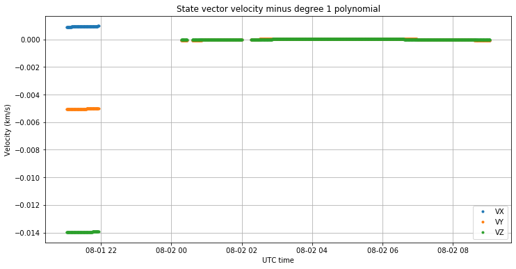
According to this data, the delta-V in ICRF coordinates was
[-0.96498824, 5.00862308, 13.94448455] m/s
The velocity-normal-binormal (VNB) reference frame is more common to express these manoeuvres. By performing an appropriate rotation we obtain the delta-V in VNB coordinates, which is
[ 5.70307085, 10.72123959, -8.54377911] m/s
The norm of the delta-V is 14.85 m/s.
When the delta-V is observed from Earth as a change in the Doppler shift, only the projection of the delta-V vector onto the line-of-sight vector joining the spacecraft and Earth can be seen. This projection is 4.28 m/s. Since the downlink signal is at 8431 MHz, we expect to see a change in Doppler of -120.2 Hz.
Doppler data was recorded by Edgar and Paul, using their own stations, and by James with the Bochum antenna. Here I am using the Doppler data kindly provided by Paul. After subtracting a degree 2 polynomial fitted to the data before TCM-1, in order to remove the Doppler due to the spacecraft’s orbit and Earth’s rotation, we obtain the figure shown below. Paul’s data has a precision of one second and one Hz, which causes the jagged appearance of the plot.
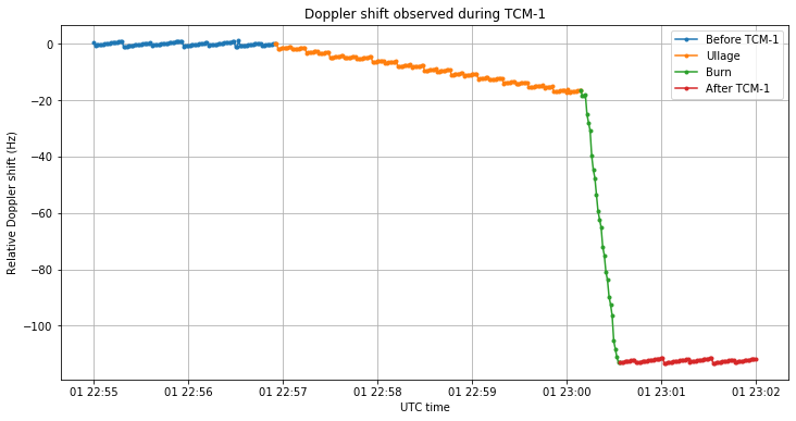
We can observe four distinct zones. First, there is a zone shown in blue which corresponds to the Doppler shift before TCM-1. We have a shift of 0Hz in this zone. Next, we have an orange zone with a shallow slope of -0.086Hz/s. This zone lasts for 194 seconds and the Doppler changes by -16.4 Hz. Then we have a steep slope shown in green. The slope is -4.36Hz/s and lasts 25 seconds, for a Doppler change of -95.3Hz. Finally, we have a red zone after the TCM-1 where the Doppler remains constant.
The green zone corresponds to the actual TCM-1 burn, and I believe that the orange zone corresponds to the firing of ullage motors to prepare the main burn.
The total change in Doppler is -111.7Hz, which is a bit less than the -120.2Hz we expected. I’m not sure where the difference comes from. I am assuming that the ullage motors and the main burn both happen along the same vector, but note that this doesn’t really matter, because the projection onto the line-of-sight vector is linear. I haven’t taken into account light-time delay to the spacecraft when computing the line-of-sight, but I don’t think this makes a large difference.
Maybe the telemetry orbit state vectors are based on a planning for TCM-1, rather than on the actual performance of the burn, since state vectors including the delta-V were available as soon as the telemetry signal came back on the high-gain antenna. We will see if in the future the state vectors change slightly as the Chinese DSN determines accurately the achieved delta-V.
Assuming that the ullage and main burns are aligned (here this matters), from the Doppler data we can compute an acceleration of 0.538m/s² for the main burn (this refers to the spacecraft acceleration, not to the acceleration projected onto the line of sight). The Chinese media state that TCM-1 was a short test firing of the main 3kN thruster in order to characterize its performance. The mass of Tianwen-1 is around 5000kg, so a 3kN force would produce an acceleration of 0.6m/s², which matches more or less our results.
Observe that according to our data, the 3kN thruster underperformed slightly, so this may justify why the observed Doppler shift was a bit less than what computed from the state vectors.
The Chinese news say that the thruster was fired for 20 seconds at 07:00 Beijing time (23:00 UTC), so this also matches our observations. In fact, the light-time to the spacecraft is already 10.14 seconds, and Paul data indicates that the start of the main burn was observed at around 23:00:09, so it may well be that the start of the main burn happened exactly at 23:00:00.
I haven’t seen any details about the ullage motors, but according to the Doppler the ullage acceleration was 0.01m/s², which corresponds to a thrust of approximately 50N. Note that for this short burn the ullage phase provided 15% of the total delta-V.
When the new trajectory described by the state vectors after TCM-1 is propagated in GMAT all the way to Mars, we see that the result is not so much different from the old trajectory. At the point of closest approach to Mars, the difference between the new and old trajectories in ICRF coordinates is
[ 1442.625535294414, 82717.67048285902, 94860.15927184373 ] km
So the closest approach to Mars is still around 3 million km. This agrees with the fact stated in the Chinese news that TCM-1 was intended as a characterization of the thruster performance in order to plan future manoeuvres accurately, rather than as an actual correction of the trajectory.
The calculations for this post have been done in this Jupyter notebook and this GMAT script.
Great stuff, as usual. Keep them honest!