W-Cube is a cubesat project from ESA with the goal of studying propagation in the W-band for satellite communications (71-76 GHz downlink, 81-86 GHz downlink). Current ITU propagation channel models for satellite communications only go as high as 30-40 GHz. W-Cube carries a 75 GHz CW beacon that is being used to make measurements to derive new propagation models. The prime contractor is Joanneum Research, in Graz (Austria). Currently, the 75 GHz beacon is active only when the satellite is above 10 degrees elevation in Graz.
Some months ago, a team from ESA led by Václav Valenta have started to make observations of this 75 GHz beacon using a portable groundstation in ESTEC (Neatherlands). The groundstation design is open source and the ESA team is quite open about this project. I have recently started to collaborate with them regarding opportunities to engage with the amateur radio community in this and future W-band propagation projects (there is an amateur radio 4 mm band, which usually covers from 75.5 to 81.5 GHz, depending on the country). As I write this, some of my friends in the Spain and Portugal microwave group are running tests with their equipment to try to receive the beacon.
On 2023-06-16, the team made an IQ recording of the beacon using their portable groundstation. They have published some plots about this observation. Now they have shared the recording with me so that I can analyse it. One of the things they are interested in is to evaluate the usage of the gr-satellites Doppler correction block to perform real-time Doppler correction with a TLE. So far they are doing Doppler correction in post-processing, but due to the high Doppler drift, it is not easy to see the uncorrected signal in a spectrum plot.
The IQ recording file is called wc_20230616_dump_1686924577.bin. It has complex int16 format. The UNIX timestamp for the start of the recording is included in the name. This corresponds to 2023-06-16 14:09:37 UTC. The spectrum of the recording is inverted because the groundstation uses an IQ mixer to convert 75 GHz to an IF, and the lower sideband of the IF is used (i.e., the local oscillator is high-side).
The GNU Radio flowgraph that I have used for Doppler correction is shown below. After format conversion (including correcting for the frequency inversion), we have the Doppler Correction block. Then there is a decimation to 2.5 ksps, which is enough to contain the CW signal with good Doppler correction. The decimation is done in two stages: decimate by 200 followed by decimate by 20. I have used my intuition when choosing the decimation factors for the stages rather than calculating an optimal distribution (the paper by Crochiere and Rabiner or the book by fred harris can be a good reference for those interested in computing an optimal chain). Between the two decimation stages there is a Rotator block that shifts the signal down by 4.5 kHz. This is done because the signal has this frequency offset. The output is written to a file, which is analysed in a Jupyter notebook.
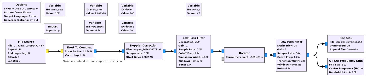
For Doppler correction I have used the following TLE. This is the closest one that I could find in Space-Track to the recording timestamp. The epoch of this TLE is 2023-06-16 07:22:53.75 UTC.
1 48965U 21059CQ 23167.30756656 .00009964 00000-0 47001-3 0 9999
2 48965 97.5997 300.9060 0010103 269.8996 90.1080 15.19632911109031
The Doppler correction needs a time offset to work well with this recording. I have determined by hand that a time offset of 3.7 seconds works best. This means that in the Doppler correction block we use 1686924577 + 3.7 as the start time. The need to add this time correction can be because of an error in the timestamp of the recording or because of an along-track error in the TLE. Along-track errors are common, specially for older TLEs, because any errors on drag or mean motion modelling accumulate as an along-track error (I’ve treated this topic in this and related posts). However, fresh TLEs are usually accurate to a couple km (an error of one second corresponds to an along-track error of about 7 km), so I think that most of the error here is on the recording timestamp.
The Doppler Correction block uses a text file that contains a time series of frequency versus time data. To generate the file I have written a Python script that uses Skyfield for the calculations.
The figure below shows the spectrum of the signal after Doppler correction. I think that the signal only appears at approximately 220 seconds because before this it is below 10 degrees elevation in Graz.
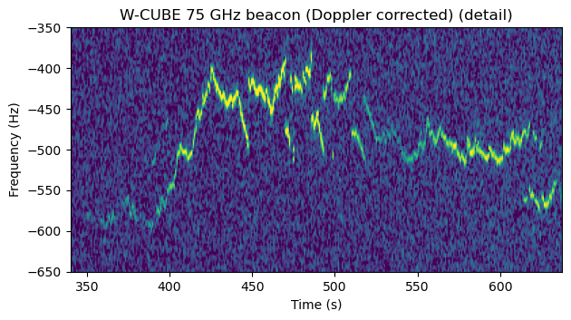
The signal drifts in frequency approximately 1 kHz throughout the pass. At these high microwave frequencies, some drift is to be expected, as 1 kHz is only 13 ppb at 75 GHz. However, it is interesting that there are frequency jumps in the signal. There is a large jump around 350 seconds, and then there are small jumps after 400 seconds and until the end of the pass. Without more information we cannot say whether the frequency instability or the jumps are caused by the satellite or by the groundstation. Maybe the jumps are caused by a jumpy TCXO. Those are TCXOs that perform their corrections in discrete jumps, which depending on the application might be noticeable. I’ve had some bad experiences with these in the past, including having to recover an image transmitted by Longjiang-2 by hand.
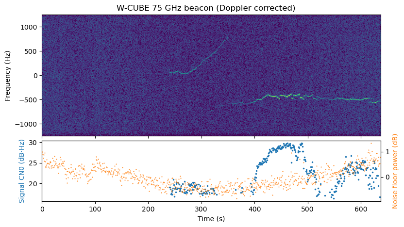
The bottom panel shows an estimate of the CN0 of the signal (in blue). There is strong fading, with the signal reaching over 30 dB·Hz at times and almost disappearing at other times. This could be due to an error in the antenna pointing or due to the attitude of the satellite. I don’t know if the satellite is attitude-stabilized. This plot of the CN0 is quite similar to the one published by ESA (thought the time axis of the ESA plot starts when the beacon begins to transmit).
The panel also shows (in orange) the relative power of the noise floor (where the average power over time is taken as the 0 dB reference). The noise floor power changes by about 1.5 dB throughout the recording, and seems to be correlated with elevation. This is to be expected, since at lower elevations there should be more noise temperature contribution from the atmosphere. It would be interesting to compare this with some of the usual models (for instance, Figure 4 in ITU-R P.372-16).
The next figure is a detail of the waterfall, in which the frequency jumps can be seen better.
All the code used for this post can be found in this repository.
One comment