Receiving HADES-D

HADES-D is the 9th PocketQube developed by AMSAT-EA. It is the first one that hasn’t failed early in the mission. Among the previous AMSAT-EA satellites, GENESIS-L and -N suffered the launch failure of the Firefly-Alpha maiden flight, EASAT-2 and HADES presumably failed to deploy their antennas, GENESIS-G and -J flew on the second Firefly-Alpha flight, which only achieved a short-lived orbit, with all the satellites reentering in about a week, URESAT-1 had the same kind of antenna deployment problem, and GENESIS-A is a short duration payload scheduled to fly in the Ariane-6 maiden flight, which hasn’t happened yet.

HADES-D launched with the SpaceX Transporter 9 rideshare on November 11. This PocketQube was carried in the ION SCV-013 vehicle, and was released on November 28. The antennas have been deployed correctly, unlike in its predecessors, the satellite is in good health, and several amateur stations have been able to receive it successfully, so congratulations to AMSAT-EA.

Since HADES-D is the first PocketQube from AMSAT-EA that is working well, I was curious to measure the signal strength of this satellite. Back around 2016 I was quite involved in the early steps of AMSAT-EA towards their current line of satellites. We did some trade-offs between PocketQube and cubesat sizes and calculated power budgets and link budgets. Félix Páez EA4GQS and I wanted to build an FM repeater amateur satellite, because that suited best the kind of portable satellite operations with a handheld yagi that we used to do back then. Using a PocketQube for this always seemed a bit of a stretch, since the power available wasn’t ample. In fact, around the time that PocketQubes were starting to appear, some people were asking if this platform could ever be useful for any practical application.

Fast forward to the end of 2023 and we have HADES-D in orbit, with a functioning FM repeater. My main interest in this satellite is to gather more information about these questions. I should say that I was only really active in AMSAT-EA’s projects during 2016. Since then, I have lost most of my involvement, only receiving some occasional informal updates about their work.

Reception set up

To receive HADES-D I used a handheld 7 element yagi antenna from Arrow Antennas and a USRP B205mini. The antenna was connected directly to the USRP with about one metre of coaxial cable. I selected an almost overhead pass on 2023-12-09 and received the pass from a relatively clear location close to home (this is where I usually do portable satellite operation). The pass that I chose was also observed by SatNOGS in observations #8678955 and #8674584.

Since I wanted to have some kind of absolute amplitude calibration, I connected a 50 ohm dummy load to the USRP instead of the antenna for some seconds at the beginning and end of the recording. With a knowledge of the USRP noise figure, we can calculate the absolute power for these parts of the recording and scale everything accordingly, assuming that the gain is reasonably stable.

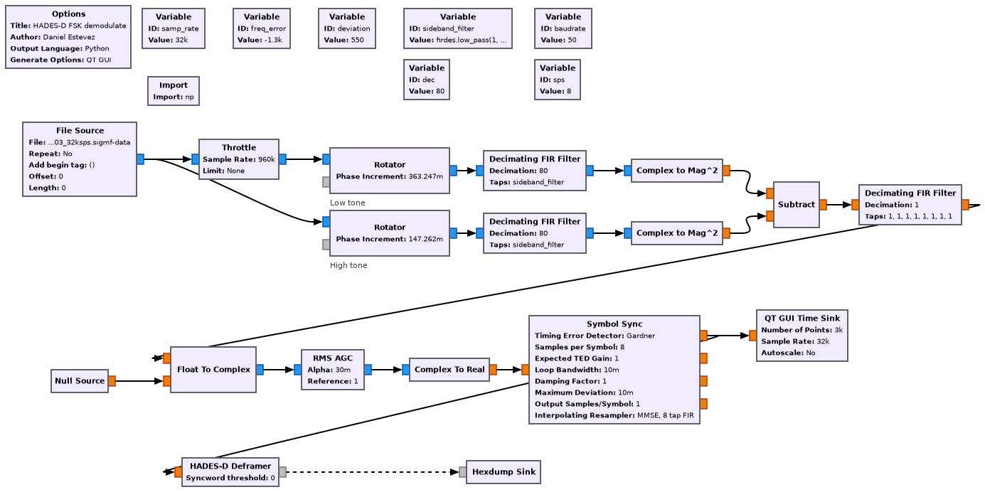
I used this GNU Radio flowgraph to perform the recording.

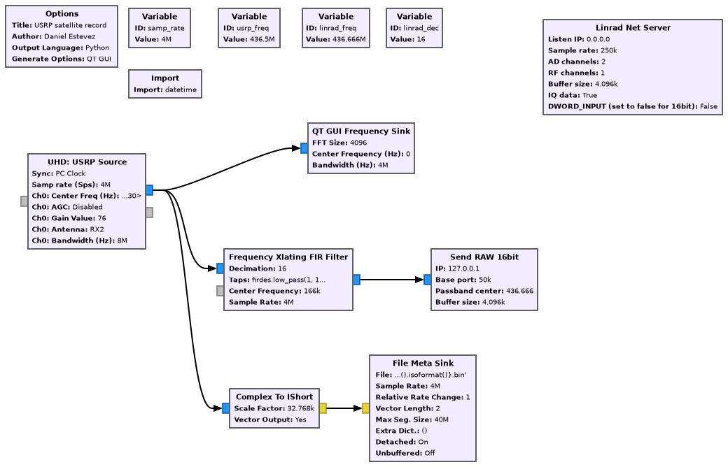
This records 16-bit IQ data at 4 Msps at a centre frequency of 436.5 MHz, so all the 435 – 438 MHz amateur satellite band is recorded. A File Meta Sink is used to record the timestamps from the USRP, which has been set using the PC clock, which was synchronized using NTP. I am using Linrad as a waterfall display. The flowgraph uses gr-linrad to send 250 ksps IQ data to Linrad centred on the HADES-D 436.666 MHz frequency. This is used to see the signal in real time and adjust the antenna pointing based on signal strength.

I used the TLE in this Libre Space forums post by Jan van Gils PE0SAT for antenna pointing. It was the best I had at the time, but when doing Doppler correction in post-processing it turned out to be wrong by about a minute.

A few minutes into the pass, the GNU Radio flowgraph stopped receiving samples. I think that the USB connector on my laptop wiggled too much. It’s been a while since the last time I did satellite reception with a laptop on the street, so I wasn’t operating as smoothly as I used to. I resumed the GNU Radio flowgraph, having lost about a minute of data. Unfortunately the Linrad network connection doesn’t like to be killed. The Linrad Net Server block spawns a TCP server at a particular fixed port, and if you kill it while there is an active connection, the kernel holds the port as busy for a long time after the process is killed. If you try to restart again, you get an error. So I had to disable the Linrad Net Server and do without using Linrad for the second part of the pass. I still had a spectrum plot of the full 4 MHz in GNU Radio, but this isn’t too good to see what is happening. So my antenna pointing might have not been the best, as I continued pointing by following the Gpredict skyplot instead of by optimizing signal strength.

Doppler correction

I did Doppler correction in post-processing, with the Doppler Correction block in gr-satellites. I have added to gr-satellites a Python script that generates the required frequency versus time text file from a TLE. This is basically the same script that I used for W-Cube.

I used the same TLE as for antenna pointing:

1 98981U          23342.52083333  .00000000  00000-0  33505-3 0    08
2 98981  97.4806  54.6245 0013454 198.3717 152.3026 15.15452664    08

However, I found that to get a good correction I needed to shift the TLE in time by 62 seconds. The HADES-D transmit frequency is not very stable, so part of the TLE time shift might be absorbing some transmitter frequency drift (and the transmitter drift could also have affected the generation of this TLE, which was done by fitting a Doppler curve).

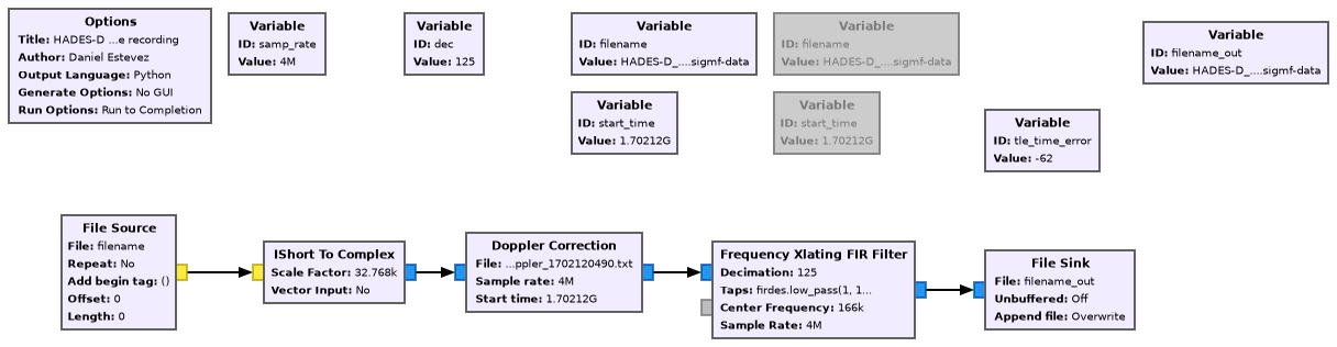
I used the following GNU Radio flowgraph to perform the Doppler correction and to decimate to 32 ksps.

Waterfall analysis

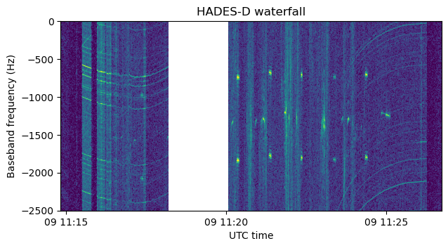
The following plot shows the waterfall of the recording around the HADES-D signal. The baseband frequency is centred on 436.666 MHz and includes Doppler correction. We can see some telemetry packets. These use 50 baud FSK with a deviation of approximately 550 Hz, so with this FFT resolution the two FSK tones are visible.

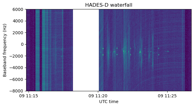
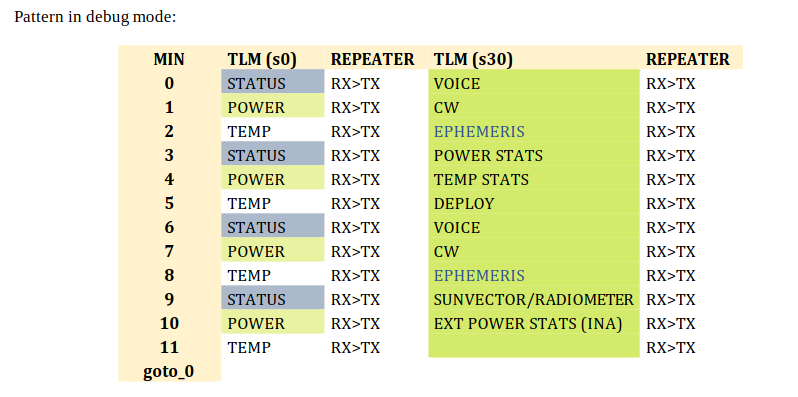
Between the FSK transmission we can see signals from the FM repeater. I think it was being commissioned during the Saturday morning in which I performed the reception. The HADES-D documentation gives the following schedule for the operation of the radio. In summary, a telemetry packet (which lasts a few seconds) is transmitted at the beginning of each minute no matter what. After this, if there is enough signal in the FM repeater receiver to active the squelch, it becomes active for the rest of the minute. If not, by the 30 seconds mark another telemetry packet, or an FM voice or CW beacon, is transmitted.

In this case we can see a CW beacon at 11:25 UTC, because the FM repeater stops being used, but before this we see the FM repeater being activated each minute.

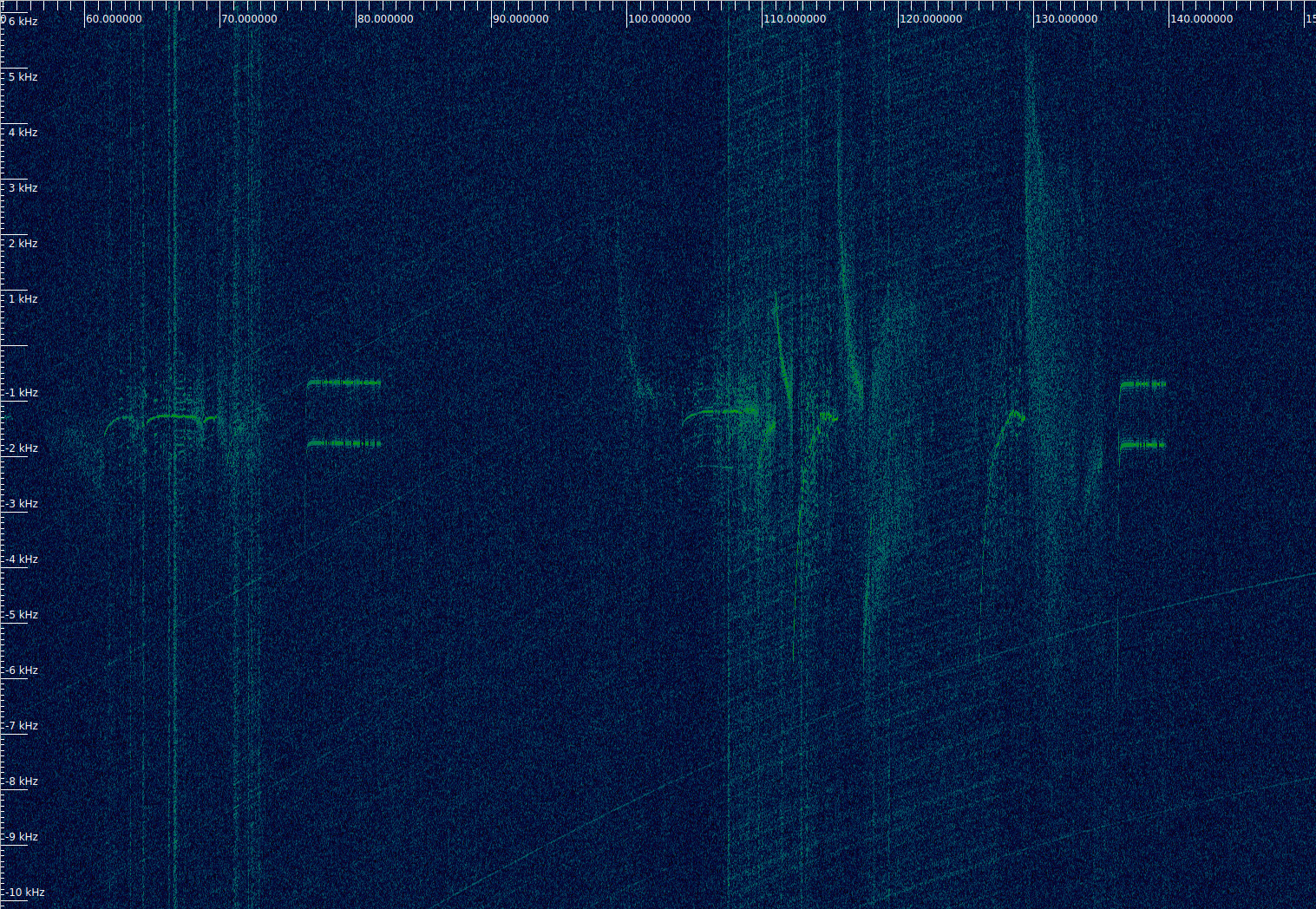
The FM transmitter on HADES-D makes a clearly noticeable chirp whenever it starts transmitting. The is both visible in the FSK telemetry transmissions and in the FM repeater. The chirp is usually an up-chirp, but occasionally some FM transmissions have a down-chirp. When the FM repeater is used, it switches on and off a number of times, perhaps because the transmitting stations key off, or because the squelch triggers due to fading. This causes a rather jumpy frequency behaviour, as illustrated by this Inspectrum waterfall. Definitely, the radio isn’t working too well. I wonder if the engineering model behaves in the same way.

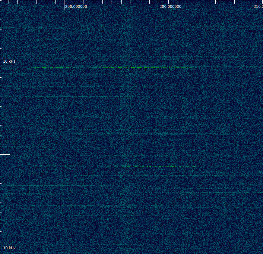
Another interesting note is that the CW transmission isn’t actually CW. It is made by shifting the signal approximately 10 kHz up in frequency in the gaps between the CW dits and dahs (this is sometimes called FSK-CW). Even though such a shift seems excessive, I guess it is okay, because a satellite with an FM voice downlink is supposed to occupy 12.5 kHz of spectrum anyway.

Absolute power calibration

I’m using an 8192 FFT with a Blackman window to study the signal. To perform an absolute power calibration, I have measured the average power in each FFT bin when the 50 ohm load was connected to the USRP at the beginning and end of the recording. The two measurements (beginning and end) are within 0.36 dB of each other, so the gain seems reasonably stable. I have simply taken the average of these two measurements for the power calibration and normalized the waterfall so that the average power of each FFT bin with the 50 ohm load is one.

FSK signal analysis

I have decided to measure the signal strength using only the FSK transmissions. Since they occupy much less bandwidth than the FM transmissions, their SNR is easier to measure. The following shows a waterfall with a narrower frequency range, where the two FSK tones as well as their spreading due to the 50 baud modulation can be seen well.

An interesting thing that can also be seen in this waterfall is that every time that the transmitter is active its frequency keeps decreasing slightly. This is best seen in some of the FSK tones and in the CW transmission. This might be due to a thermal or bus voltage effect.

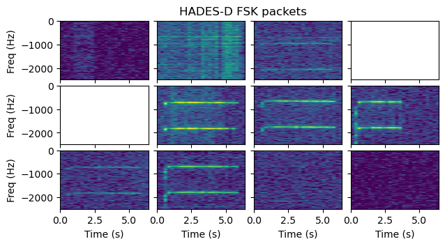
Using the fact the FSK packets are transmitted exactly every minute, it is easy to select the parts of the waterfall that contain FSK packets. The following shows all the slots where an FSK packet would be transmitted. There are 4 strong packets and 2 much weaker packets visible. One of the packets is shorter, but this is normal, because there are different telemetry packet types with different lengths.

I have detected the frequency of the low FSK tone in each of the visible FSK packets and selected windows to sum up the power of the two tones. These are shown below in red. The noise floor is measured over the rest of the FFT bins in this 2.5 kHz slice, which are marked in grey.

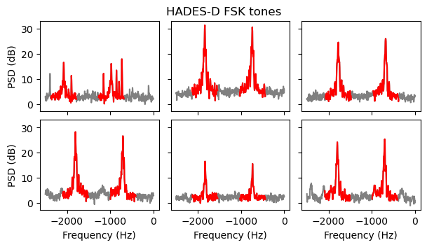
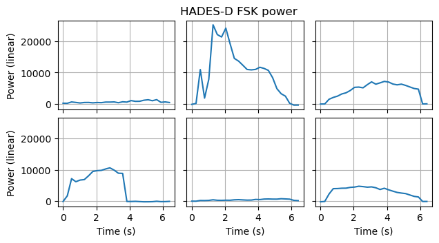
The power of the FSK signal is computed by adding the power in the regions marked in red, taking the average of the regions marked in grey to estimate the noise floor, and subtracting from the sum the noise floor estimate times the number of FFT bins marked in red. The plot below shows the power of the FSK signal over time in each of the FSK packets. The plot confirms that the noise floor has been estimated correctly, since the power before the beginning and after the end of the transmission is very close to zero.

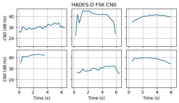
A CN0 estimate can be calculated and plotted from the FSK power and the noise floor estimate. The CN0 ranges between 40 and nearly 50 dB·Hz for the strong packets. In the weak packets it is around 30 dB·Hz, but this estimate should not be trusted much.

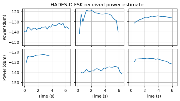
Using the absolute power calibration and assuming that the USRP has a noise figure of 5 dB (which is probably within 1 dB of its true value), we can convert the power measurement to dBm. These estimates have an accuracy of maybe 2 dB. We see that the strongest packet has a maximum power of -120 dBm.

Now we can do some ballpark estimates to get the EIRP of the satellite transmitter. This is like running the link budget in reverse. The distance to the satellite when the strongest packet was transmitted as 569 km. I don’t know the gain of my 7 element yagi, but I’m going to assume a gain of 12 dBi to account for some pointing loss (a 7 element yagi usually has a gain around 10.5 to 11.5 dBd, which is equivalent to 12.65 to 13.65 dBi). Putting all of this together with the -120 dBm power measurement gives us an EIRP at the satellite of 8.4 dBm.

This estimate has probably a few dB of error, but still places some constraints on the power transmitted by the satellite. Given that I have selected the strongest packet, the antenna pattern is favourable, or at least not unfavourable (in contrast, the fifth packet in the plot above is an example of antenna pattern or polarization null, since it happens between two much stronger packets). I haven’t found documentation stating what the satellite output power is, but I would find hard to believe that it is 20 dBm or more. With the estimate of 8.4 dBm EIRP that I have obtained, I would think that the transmit power is 13 dBm or less.

Telemetry decoding

The HADES-D FSK waveform is somewhat unusual because its deviation is much larger than the baudrate. In this situation, an FSK demodulator based on quadrature demodulation, such as the one included in gr-satellites, works badly. This is because the signal needs to be quadrature demodulated in a bandwidth that contains the two tones. This lets too much noise in, and quadrature demodulation is a nonlinear process, so we lose a lot of SNR. An alternative demodulation strategy consists in filtering each of the two tones, measuring its power, and subtracting the two powers. The bandwidth of the filters needs to be comparable to the baudrate to avoid losing SNR.

In the case of HADES-D there is an extra difficulty, because its frequency is not stable (and also currently the TLE has a large error). A reliable demodulator would need to detect and track the frequency error. There are many good techniques to do this, but they make the demodulator more complex.

In this case I have kept it simple, and performed demodulation without any kind of frequency tracking. I have already adjusted the TLE error, and in the demodulator I am adjusting the remaining frequency error by hand. The demodulator architecture follows exactly what I have explained above. The bandwidth of the filters is +/- 200 Hz, so any frequency error larger than this will make the demodulator fail.

I have added the flowgraph above as an example in gr-satellites. I don’t know how useful it will be in practice to run in an automated way, due to its small frequency error tolerance.

I have also implemented a deframer for gr-satellites. The deframer detects the packet type, which is required to crop the packet to its correct length, and performs CRC-16 checking and descrambling. HADES-D is unusual because the CRC-16 is computed over the scrambled data, and the CRC itself is not scrambled. Therefore, the CRC should be checked before descrambling.

The CRC algorithm is the usual CRC-16-CCITT-FALSE. The implementation in the official AMSAT-EA software is rather interesting. It is a byte-by-byte calculation that doesn’t use a table and only performs 5 XORs and a few shifts per byte. I don’t know if I have seen this kind of implementation before, but it looks quite good for microcontrollers (the implementation comes from the flight software).

The scrambler is an unusual thing, because it is a multiplicative scrambler, but the shift register is reset to a certain value at the beginning of each packet. The documentation mentions that the reset value is 0x2C350000, but it is not very detailed regarding bit order, so it’s difficult to understand exactly what this means. Moreover, it is impossible to implement the scrambler just by looking at the documentation, because there is a bug in the software (both in the satellite and the official decoder). Some loops say for (int b = 7; b > 0; b--) instead of for (int b = 7; b >= 0; b--), so the LSB in each byte is not scrambled as a consequence. This was first noticed by Andy UZ7HO when he implemented his own decoder for one of the previous AMSAT-EA satellites. Moreover, the reset value is set to be 0x2C350000 both in the documentation and code, but only the 17 LSBs of this value are used, so the reset value could more simply be said to be 0x10000, which is what I have used in my implementation.

There is no FEC, which makes the decoding process quite unforgiving. Decoding fails if there is a single bit error, which could happen due to frequency error or due to a fade in a long packet (there are some packets which are 23.2 seconds long).

When the decoder is run on the second part of the recording, it is able to decode the 4 strong packets. The weak packet has a couple of bit errors, so decoding fails. These are the hex dumps of the decoded packets.

0000: 38 2a aa 0e 00 4b 00 0c 00 00 1e 03 11 00 01 00 
0010: 00 ff 02 11 00 01 00 00

0000: 18 07 00 2e 00 00 00 9b b6 6b 69 02 94 53 40 0f 
0010: fa 01 af 00 00 69 00 00 

0000: 28 4c 4c 48 4c ff 3e 41 46 40 4a 

0000: 18 0c 05 18 63 00 00 7b b6 6b 68 f9 a3 b3 3f 0f 
0010: f7 01 f9 00 10 6b 00 00 

The 4 MSBs in the first byte of each packet indicate the packet type. Here we have types 1 (power), 2 (temperature), and 3 (status). Their transmission order matches the schedule in the documentation. Taking into account the fact that the last packet is accompanied by a CW beacon, we see that the first of these packets corresponds either to minute 3 or minute 9.

FM repeater commissioning

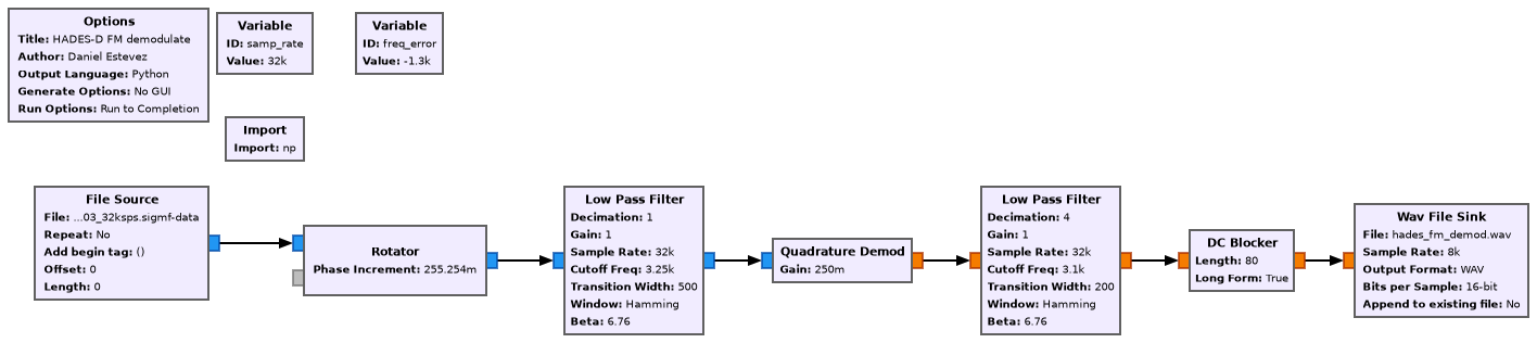
I have used the following GNU Radio flowgraph to demodulate the FM repeater audio.

Below are the audio excerpts in which the FM repeater is active. We can hear EB1AO (who is one of the satellite command stations) and an EA4 station (I can’t make out his full callsign) complete a QSO by exchanging 59 reports.

The first excerpt is strange, because it seems it’s other people speaking, and perhaps transmitting through the satellite just accidentally. I’m not even sure that the language is Spanish. It almost seems Italian.

The second excerpt is more of the same.

In the beginning of the third excerpt I think it’s the same strange stations as before, but then we can listen EB1AO calling CQ sat. The EA4 station replies calling EB1AO, and EB1AO calls CQ sat again.

In the fourth excerpt EB1AO is repeating his callsign and giving the signal report (59) and locator (IN52). Then the EA4 station replies, but his callsign fades away.

In the last excerpt we can hear the EA4 station confirming that he has copied the data and giving a 59 report from locator IN80.

By listening to this, I get the impression that these two stations could receive the satellite better than I. They seem to acknowledge pieces of data that were completely faded in my recording. I imagine that they have longer yagis on a fixed station. Having 4 dB more of gain or so would make a huge difference, due to the nonlinear relation between output SNR and input SNR in an FM demodulator.

I wonder how well the satellite was working from the point of view of these two stations. They take slightly more than 2 minutes to complete the contact. A quick contact on a busy FM satellite with only signal reports and locators exchanged can easily be completed in 30 seconds. On the one hand, if they were the only two stations supposed to be testing the FM repeater, they could do it more leisurely. But I’m not sure if the squelch is opening reliably for them or if the telemetry breaking in every minute is too much of a problem.

Another remark is that EB1AO seems to have a fully quieting signal at the input of the FM repeater, because the downlink spectrum looks clean. Only the voice formants are visible. On the other hand, for the EA4 station the downlink spectrum doesn’t look clean, and in the FM demodulated audio there is always much more background noise. Maybe his uplink signal is already like this, or maybe he isn’t reaching the repeater input with enough SNR for a fully quieting signal.

Conclusions

The questions with which I began this post were whether a PocketQube like HADES-D can be a viable amateur FM repeater satellite and whether a PocketQube has enough power budget and size to be useful for some practical application. With the antenna I used to receive this pass it was quite difficult to copy the FM audio. I could only understand it after playing it back for several times at home. Probably I wouldn’t have managed to complete a contact under these conditions (though it’s also been a while since I last operated FM satellites and my skills are a bit rusty).

I get the impression that the two stations involved in the contact had larger antennas and could copy the FM audio much better. Although this recording is just a single data point, and more usage will tell the full story, it seems that HADES-D is not a viable satellite for operating on the street with handheld antennas, as Felix and I used to do. On the other hand, larger fixed stations probably have enough link budget to use it. Maybe this is fine. In another experiment I did on this blog, I struggled to receive the GreenCube satellite (note that I did that recording in a much more noisy location). Yet, with time, the digipeater on this satellite has proven to be quite popular because the satellite is in MEO orbit and has a large footprint. Even if it’s not easy to receive with a small antenna, larger stations use it regularly.

Code and data

The IQ data used in this post has been published in the Zenodo dataset Recording of HADES-D satellite. The GNU Radio flowgraphs and the Jupyter notebook can be found in this repository.