Radiometry for DELFI-PQ, EASAT-2 and HADES

On January 13, the SpaceX Transporter-3 mission launched many small satellites into a 540 km sun-synchronous orbit. Among these satellites were DELFI-PQ, a 3U PocketQube from TU Delft (Netherlands), which will serve for education and research, and EASAT-2 and HADES, two 1.5U PocketQubes from AMSAT-EA (Spain), which have FM repeaters for amateur radio. The three satellites were deployed close together with an Albapod deployer from Alba orbital.

While DELFI-PQ worked well, neither AMSAT-EA nor other amateur operators were able to receive signals from EASAT-2 or HADES during the first days after launch. Because of this, I decided to help AMSAT-EA and use some antennas from the Allen Telescope Array over the weekend to observe these satellites and try to find more information about their health status. I conducted an observation on Saturday 15 and another on Sunday 16, both during daytime passes. Fortunately, I was able to detect EASAT-2 and HADES in both observations. AMSAT-EA could decode some telemetry from EASAT-2 using the recordings of these observations, although the signals from HADES were too weak to be decoded. After my ATA observations, some amateur operators having sensitive stations have reported receiving weak signals from EASAT-2.

AMSAT-EA suspects that the antennas of their satellites haven’t been able to deploy, and this is what causes the signals to be much weaker than expected. However, it is not trivial to see what is exactly the status of the antennas and whether this is the only failure that has happened to the RF transmitter.

Readers are probably familiar with the concept of telemetry, which involves sensing several parameters on board the spacecraft and sending this data with a digital RF signal. A related concept is radiometry, where the physical properties of the RF signal, such as its power, frequency (including Doppler) and polarization, are directly used to measure parameters of the spacecraft. Here I will perform a radiometric analysis of the recordings I did with the ATA.

Recordings

The recordings are already published in Zenodo, in the following datasets:

Here I will mainly be analysing the recording from 2022-01-15. I haven’t done an analysis of the recording from 2022-01-16 with the same level of detail yet, but I will show a few new things from this recording at the end of the post.

To do these recordings I used antennas 1a and 1f. The Allen Telescope Array antennas are 6.1 m dishes with a Gregorian structure and a logperiodic feed, giving very wide frequency coverage. The feed has dual linear polarization. The two polarization channels are called X and Y, which correspond to horizontal and vertical (or maybe the other way around, as I tend to forget).

Antennas 1a and 1f in particular have “old feeds”, which have a coverage between roughly 0.5 and 10 GHz. The newer feeds, which have been installed in most of the antennas, cover between 1 to 14 GHz, with much better performance at high frequencies, due to the fact that the feed is fully cryogenic, instead of only the LNA. However, for observations in the 435 MHz amateur satellite band, the old feeds are much better (though still this is outside the design frequency coverage of the feed).

Something to keep in mind is that the ATA antennas can only track above 16.8 degrees elevation. Moreover, when tracking a TLE, tracking will start fixed at the location where the skytrack crosses 16.8 degrees elevation when the satellite rises, and will also stop at the location where the skytrack crosses 16.8 degrees elevation as it sets. Both the azimuth and the elevation of the antennas will stay fixed when this happens, so there will be a pointing error both in azimuth and elevation.

The recordings I did used a sample rate of 3.84 Msps in order to cover the full 435 – 438 MHz amateur satellite band. Besides the three satellites we study in this post, many other satellites from the Transporter-3 launch, or that just happened to be in the sky at that moment, appear in the recordings, so they could be of interest to other satellite operators. The first step in processing the data is to channelize and downsample the recording for each of the three satellites we are studying. This GNU Radio flowgraph is used to downconvert the signals from each satellite (using centre frequencies of 436.650, 436.680 and 436.895 MHz for DELFI-PQ, EASAT-2 and HADES respectively) and decimate to 40 ksps. The resulting files are analysed in a Jupyter notebook.

Doppler correction

The first step in the processing is to perform Doppler correction. One of the other things I have done with these recordings is to use STRF (see also my crash course) to measure the Doppler of these satellites and fit TLEs. The results are in this repository. Using these fitted TLEs and Skyfield, we can compute the Doppler for each of the satellites and perform Doppler correction.

When the recordings were done, the three satellites were still quite close together. In fact, their Doppler curves are only a few seconds apart, so it is difficult to tell them apart just by using Doppler measurements. On the other hand, this is helpful, because the half-beamwidth of the ATA antennas at 436 MHz is around 4 degrees, so we know that we had the three satellites close to the centre of the beam. Other satellites from the Transporter-3 launch were minutes behind these, putting them many degrees away on the sky, so they were received with the antenna sidelobes.

Amplitude calibration

The next step is to do an amplitude calibration of the 4 channels (two antennas times two polarizations), which is necessary because the electronics of each channel have somewhat different gains. In radio astronomy this calibration is usually done by observing a (mostly unpolarized) radio source that might also serve for absolute amplitude calibration. Other sources such as a satellite with a stable, circularly polarized signal, could be used as well.

In our case, we do not have such kinds of signals. An alternative way to perform the calibration is to assume that all the channels have the same noise temperature, and calibrate the amplitudes so that the noise floor level is the same in all the channels. This is just an approximation because in reality each of the channels will have slightly different noise temperatures. Also, any polarized interference or interference that is local to one of the antennas will mess up with this technique.

Without a better alternative, this is the approach that we follow here. We use a frequency segment in the DELFI-PQ channel that is clean of interference and measure the average power for each channel over all the duration of the recording. This is used to determine a constant amplitude scaling for each channel.

Waterfalls

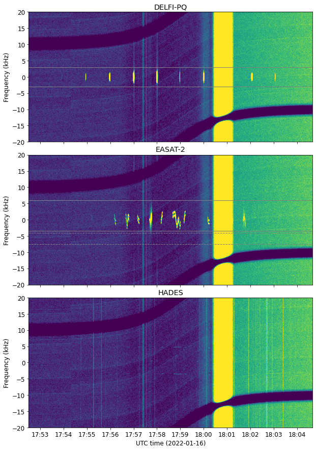
We compute waterfall data for each of the channels using an FFT resolution of around 9 Hz. Adding the calibrated waterfalls from the four channels, we obtain the Stokes I brightness for each of the satellites. This is plotted below. The dynamic range in the plot is only 5 dB, so that we can see the weak signals of HADES. The signals from DELFI-PQ and EASAT-2 saturate this scale.

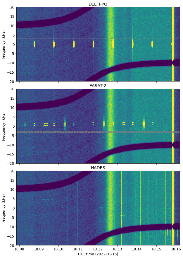
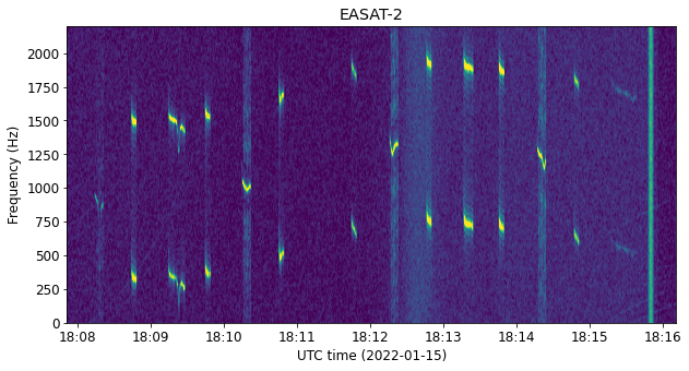
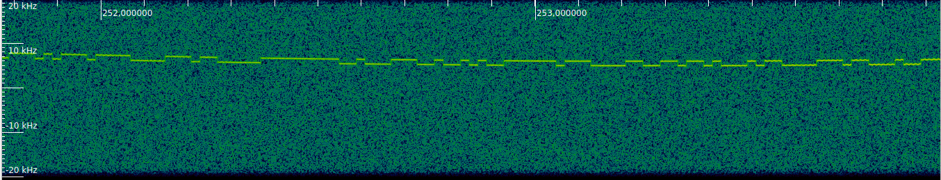
DELFI-PQ is sending a beacon packet every minute, as it usually does. EASAT-2 follows its transmission schedule, which is described in page 13 of this document. At the start of every minute (according to the on-board time, which is way off from UTC), a “fast” (short) 50 baud FSK telemetry packet is sent. Then, at 30 seconds in the minute some kind of data is transmitted. The nature of this data changes depending on the minute in question, following a cycle of 14 minutes. The transmissions we can see are the FM transmission of a voice beacon (1st, 5th, 8th, and 12th transmission), an FSK-CW beacon (3rd transmission), and the 50 baud FSK transmission “slow” (long) telemetry packet (10th transmission). The remaining transmissions we see are “fast” telemetry packets. The deviation of the FSK modulation is around 600 Hz. There is some frequency instability in the transmitter, which is best seen in the zoomed in waterfall below (which now uses a dynamic range of 20 dB). Note some rather fast occasional frequency “glitches”, besides the overall drift.

The signal of HADES is much weaker. The following zoomed in waterfall enhances it slightly (4 dB dynamic range). We can see that it follows the correct transmission schedule, albeit with a different time offset than EASAT-2 (this is just due to the on-board times of the satellites). In the waterfall we can see the FSK tones and also the carrier of the FM voice transmissions. The deviation is around 4.5 kHz, much larger than that of EASAT-2. This is by design, so it is to be expected.

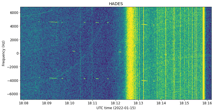
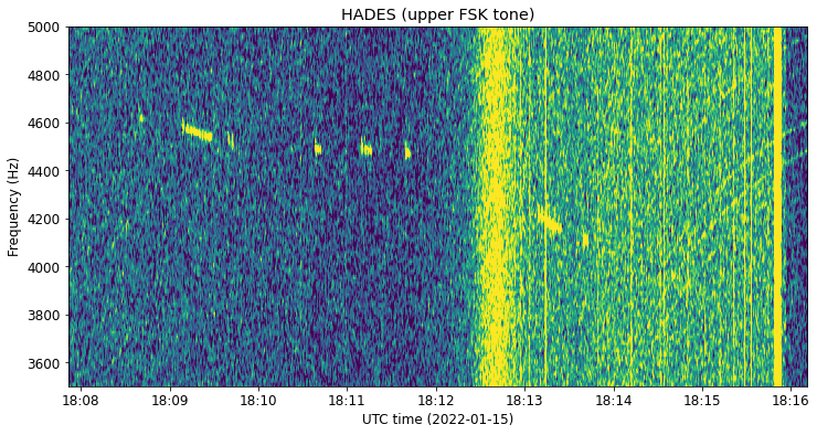
By zooming in to one of the FSK tones, we can see qualitatively the same kind of frequency drift as in EASAT-2. However, we don’t see the fast frequency glitches (though maybe this is just because the signal is too weak to see them should they happen).

Signal power

Studying the signal power is of great interest given the hypothesis that the antennas haven’t managed to deploy. Besides the fact that the gain of an undeployed antenna is much less than the gain of a properly deployed antenna, its impedance will also be quite far from the expected value. Therefore, the power amplifier might not be able to supply its full power to the antenna due to impedance mismatch. Moreover, it might happen that this impedance mismatch makes the amplifier fail (either instantly or eventually). Additionally, many more things can go wrong in the transmitter during launch, causing decreased signal levels. For instance, anything involving broken components or solder joints. Additionally, it should be kept in mind that even with failed components or broken solder joints, if the leakage of the transmit signal is enough, a sensitive instrument such as the ATA or another larger telescope might be able to detect the downlink signals.

All this makes it difficult to be sure about the exact nature of the failure just from observing the RF signal. Anechoic chamber measurements of the satellite with the antennas folded can be useful as a guide to compare with what is seen in orbit. However, these are not available for EASAT-2 and HADES.

When measuring the power of the signals of EASAT-2 and HADES, we can use the signal of DELFI-PQ as a reference. This satellite is working well and its signals are as strong as expected. We need to keep in mind that DELFI-PQ has a transmit power of 24 dBm EIRP (taking into account the gain of its dipole antenna). The transmitter of EASAT-2 and HADES only has 16 dBm of power (not taking into account the gain of the antenna).

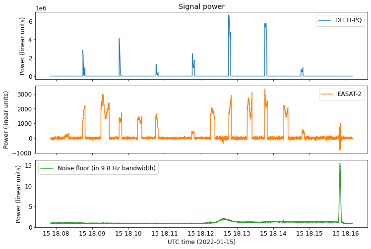
To measure the signal power of DELFI-PQ and EASAT-2, we measure the signal plus noise power in some frequency sub-bands that contain the signals of interest. These have been marked with gray lines in the waterfall shown above. Additionally, we measure the noise spectral density in the sub-band marked with dashed lines in the EASAT-2 channel. This measurement is used to subtract the noise from the signal plus noise measurement, giving us only signal power. All this is done in the Stokes \(I\) data formed by averaging the data from the two antennas and polarizations.

These three measurements are shown below. Note that the amplitude has been scaled so that the noise in an FFT bin (~9.8 Hz bandwidth) averaged over the recording duration is one. Therefore, the noise spectral density (per FFT bin) we measure is close to one, except for some increases due to interference.

Now we can turn this data into an estimate for the CN0 of the signals. For the noise spectral density N0 here we use the average over all the recording, rather than the time varying measurement done above. This is better suited to our purpose of studying the signal power, since changes in the noise floor due to interference won’t impact our measurement. In this respect, N0 is just used as a constant for power scaling, which can be related to the noise temperature of the instrument.

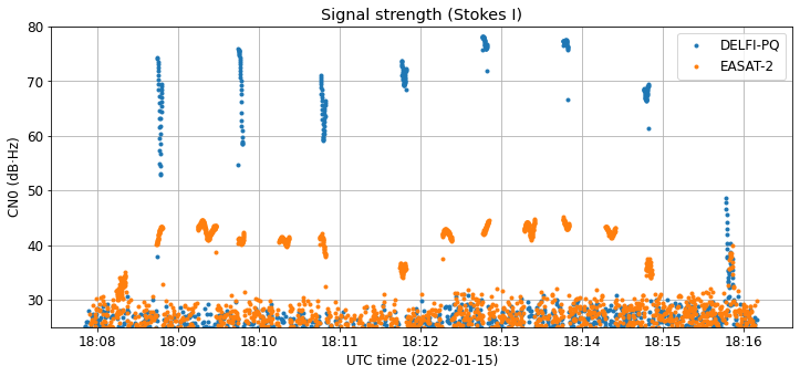
We see that the signals of DELFI-PQ are between 70 and 80 dB·Hz, while the signals of EASAT-2 are between 40 and 45 dB·Hz. Additionally, EASAT-2 has between 30 and 35 dB less power than DELFI-PQ. If we assume that EASAT-2 is transmitting at its full 16 dBm power, the conclusion here is that its antenna has a gain on the order of -20 to -25 dBi, because DELFI-PQ has an EIRP of 24 dBm. Note that this EIRP figure for DELFI-PQ, which has a dipole antenna, probably refers to the peak antenna gain (which should be around 2 dBi), so in reality the EIRP we’re seeing from DELFI-PQ could be a few dB less than 24 dBm.

It’s worth to compute the link budget for DELFI-PQ to check that our measurements are on the correct ballpark. However, we do not have any data for the performance of the ATA antennas at 436 MHz, since the feeds are only specified down to 500 MHz. Assuming a system temperature of 100 K (the system temperature at higher frequencies is maybe 30-50 K) and an antenna gain of 26.7 dBi (which gives a G/T of 6.7 dB K⁻¹), for a distance of 700 km (corresponding to the closest approach) and a transmitter of 26 dBm EIRP, we would see an SNR of 82.2 dB·Hz. Here we have taken into account the fact that here we are using Stokes \(I\), so the noise power is double from what we would have in a single-polarization system. The maximum power we’re seeing in our measurements of DELFI-PQ is slightly less than 80 dB·Hz, so everything seems reasonable giving or taking a few dB.

The measurement of the signal power of HADES can’t be done in the same way, because the signal is much weaker. We do a single measurement by averaging over the duration of one of the packets that seems strongest in the waterfall. The figure below shows the PSD of this packet.

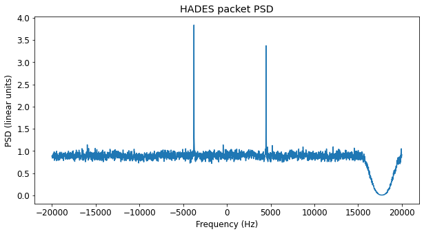
Measuring the signal plus noise about the two FSK tones, and taking some free portion of the spectrum to measure noise spectral density, we get a CN0 of 22.9 dB·Hz. This is 20 dB weaker than EASAT-2, and all in all, between 50 and 55 dB less than DELFI-PQ. These losses might seem too high to be only caused by the geometry of the undeployed antennas. It might be the case that the power amplifier is not delivering the power it should, or perhaps it has failed completely. AMSAT-EA thinks that the reason for the signal power difference between EASAT-2 and HADES is that the antennas of the two satellites were folded in a somewhat different manner, but there are no on-ground measurements of the effects of this difference.

Polarization

One of the advantages of using the Allen Telescope Array is that it is a dual polarization instrument, and can be used to measure the polarization of the RF signal. This can give us interesting information about the antennas and the attitude of the satellite. Many small satellites have dipole or monopole antennas, which are linearly polarized. The polarization angle of the RF signal will depend on the angle with which the antenna is seen from ground, and will change as the satellite rotates.

Other satellites have turnstiles or other kinds of circularly polarized antennas. Typically, these only have their intended circular polarization when seen from boresight. Seen from the side they often have linear polarization, and from the back they will typically have the opposite circular polarization. This topic has already appeared in my studies about the polarization of Chang’e 5, although in this case we had the additional difficulty that we didn’t now the types of antennas used nor how they were placed in the spacecraft body.

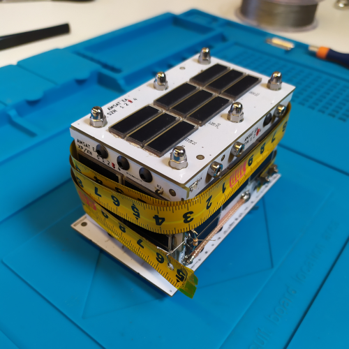
EASAT-2 and HADES were launched with their antennas wrapped around the spacecraft body, as seen in this image. The antenna for the 436 MHz downlink is a monopole built with metric tape. If the antennas were correctly deployed, we would expect to see linear polarization. However, with the antennas folded in this way, the polarization will be some kind of elliptical polarization that depends on the angle with which we view the spacecraft.

EASAT-2 with folded antennas (taken from its SatNOGS DB entry)

To measure the polarization correctly we need to do some calibrations. Gains were calibrated as indicated above. For polarimetry it is important that the gain calibration is accurate, since any gain errors will make Stokes \(I\) leak into Stokes \(Q\). Another parameter that needs to be determined is the phase offset between the X and Y channels of each antenna. This is a constant for each antenna that is relatively stable over frequency. Without knowing this offset, it is impossible to separate the cross-correlation of the X and Y channels into Stokes \(U\) and \(V\).

There are several methods of calibrating the X-Y phase offset. The most straightforward is to observe a linearly polarized source, for which we know that \(V = 0\). Note that this only solves the phase offset up to a 180º ambiguity, since we don’t know whether \(U > 0\) or \(U < 0\) unless we know the polarization angle of our calibrator source. Additionally, the polarization angle of the calibrator shouldn’t be 0 or 90 degrees, since in this case we wouldn’t see anything in the correlation of X and Y.

In radio astronomy other approaches are followed, since sources are not strongly polarized (typically 10% or less polarization degree), so that any polarization leakage can swamp out the source polarization. Therefore, polarization leakage is typically determined previously or together with the X-Y phase offset. Since we’re dealing with fully polarized signals, we do not need these additional complications, and in fact we will not calibrate and remove the polarization leakage.

Here DELFI-PQ is again useful as a reference, since its downlink antenna is a dipole, with linear polarization. We will use its signal for X-Y phase offset calibration, by taking a strong packet, and determining the phase offset that makes \(U > 0\) and \(V = 0\). Note that the choice of \(U > 0\) is arbitrary, so the sign of \(U\) and \(V\) in our results could be wrong, as well as the sign of the polarization angle that we measure.

Another effect that involves the polarization is the Faraday rotation in the ionosphere, which at 436 MHz is significant. We will ignore this, which means that we will not be able to determine absolute polarization angles of the transmitted signal (astronomers like to think that the ionosphere rotates their telescopes). The change in Faraday rotation as the satellite crosses the sky is also important, but this happens relatively slowly, so it is of no concern for the interpretation we will do of our results.

Finally, some care needs to be taken with this results, since the instrumental polarization of the ATA antennas depends on the position of the objects within the antenna beam. More information can be seen in ATA memo 88 about wide field polarization calibration. In our case, we do not know if the satellites were exactly in the centre of the beam, due to possible errors in the TLEs and the fact that the tracking of fast LEO passes may not be as accurate as the tracking of objects moving at sidereal rate (although the ATA antennas can track most LEO passes). Still, judging the results we get from DELFI-PQ, our measurements seem of reasonable quality.

Besides calibrating the X-Y phase offset, we consider the frequency sub-band in the EASAT-2 channel that we used to measure noise. Taking this sub-band we can measure the Stokes parameters of the noise spectral density. The \(I\) accounts for the noise temperature of the system, but \(Q\), \(U\), \(V\) are non-zero because of instrumental polarization leakage and perhaps polarized interference. This is then subtracted from the Stokes parameters of the signal plus noise measurements of DELFI-PQ and EASAT-2 in order to cancel out the contribution from the noise. This correction is only significative in the case of EASAT-2, since the signal of DELFI-PQ is much stronger than the noise.

The figure below shows the Stokes parameters and polarization angle of the DELFI-PQ packets. In order to show each packet in detail, only time segments around each of the seven packets in the recording have been plotted. The legend for the plot is as follows: Stokes parameters are referred to the left axis, using blue for \(I\), orange for \(Q\), green for \(U\), and red for \(V\); the polarization angle is referred to the right axis and plotted in grey. The upper and lower rows show the data for each of the two antennas. We can see that they are quite consistent.

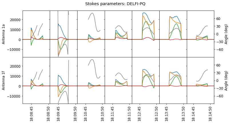
What we see here is reasonable for a linearly polarized satellite that is tumbling. Stokes \(V\) is very small, indicating little circular polarization. Inside each packet, which lasts for about 4 seconds, we can see the polarization angle changing roughly as a sinusoid. This is to be expected. For a short timescale, we can assume that the satellite is rotating with constant frequency about a constant axis. Then the angle with which we would see the antenna on ground follows a sinusoid whose frequency equals the rotation frequency and whose amplitude and offset can be determined from the relative angles between the antenna axis, the rotation axis, and the line of sight.

Glancing at the plots, we can see that the rotation period is on the order of perhaps 6 to 10 seconds. Moreover, the amplitude and offset of the sinusoid change in each packet, indicating a changing geometry for the tumbling of the satellite. Keep in mind that part of this change is due to the rotation of the line of sight vector with respect to the inertial frame as the satellite crosses the sky.

Now, for EASAT-2 we get the following plot, which shows all the packets present in the recording, using the same kind of legend. Again, we see good consistency between each of the two antennas.

The results are now much harder to interpret. We see that now \(V\) is non-zero and changes sign depending on the packet. This shows the presence of circular polarization, which supports the idea that the antennas are not deployed correctly. The curves traced by each of the Stokes parameters are much less regular than for DELFI-PQ. Without a knowledge of the polarization radiation pattern of the folded antennas (which could be measured in an anechoic chamber), it isn’t easy to understand what is going on here. Still we can say something very approximate about the tumbling rate of the satellite, looking at the time scale of the polarization variations within each packet. These seem to indicate a tumbling rate similar to that of DELFI-PQ, with a period of perhaps 5 to 10 seconds.

Since the signal of HADES is very weak, I have not attempted to study its polarization, but it would be interesting to check if there is a significant circular polarization.

Some signal aspects in the 2022-01-16 recording

Here I comment on some new signal aspects that appeared in the recording from 2022-01-16. The waterfalls for the three satellites corresponding to this recording are shown here. We can see that DELFI-PQ and HADES look roughly the same as the previous day. However, EASAT-2 has a very large frequency instability.

This is seen better in the plot below, which shows only the time and frequency range over which there are packets from EASAT-2.

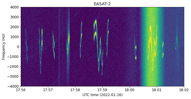
Zooming in to the long transmission around 17:59 UTC, we see the following. This is a 50 baud FSK packet. The drift is as high as 3 kHz. Additionally, we can see that at times the FSK tones are much wider than expected, and indeed with this FFT resolution their power seems to split into two sidebands. Compare the tones around 17:58:51, which are normal, with those at 17:58:56, which are anomalous.

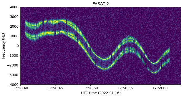
The reason for this can be seen better in inspectrum, where we can play interactively with the FFT resolution. The figure below shows the FSK tones for one of the good parts of this packet. Note that the tones are clean and they show up as straight lines.

Now, this is how one of the bad parts of the packet looks like (click on the image to see it in full). The FSK tones have a superimposed sinusoidal frequency ripple. The frequency of this ripple is approximately 75 Hz. The cause of this ripple is not known, but this is something that didn’t happen during the previous observation.

This ripple comes and goes in a smooth fashion, slowly increasing in amplitude over the course of 5 seconds or so, and then decreasing again until it disappears. This happens throughout all packets in the recording. In the FM voice beacons it can be seen in the carrier.

It is not known if the much larger frequency instability and the presence of this ripple are related or if they are two independent problems. Additionally, this ripple hasn’t been observed in HADES, although if it were present it would be harder to see it, due to the much weaker signal.

Other ideas

Since the recordings have two antennas, interferometry could be used to try to distinguish the spacecraft for orbit determination. The signals are only a few kHz wide, so we would need to do narrowband interferometry (see Section 13.7.1 in the book by Moyer). This is equivalent to measuring the Doppler difference between the two antennas. The baseline formed by antennas 1a and 1f is only 79 m long, and is roughly oriented north-south, the same as the direction of the pass of these satellites.

I haven’t thought carefully whether this narrow band interferometry gives results of any interest. I have done some simplified calculations for a satellite with orbital velocity \(v\) and height \(h\) passing directly overhead a baseline of length \(l\), and with the orbital plane containing the baseline. Around the closest approach, to first order estimate the narrowband interferometry gives \(vl/h\). This means that it is not sensitive to along-track errors, and is only able to estimate the orbital velocity and height, which are often better constrained in terms of the timings of successive passes (since errors in the orbital period accumulate over time). Higher order terms might have more interesting information, however.

Data and code

The recordings used here have been linked at the beginning of the post. The GNU Radio flowgraph and Jupyter notebooks can be found here.