An STRF crash course

Recently, the STRF satellite tracking toolkit for radio observations by Cees Bassa has been gaining some popularity. This toolkit allows one to process RF recordings to extract frequency measurements and perform TLE matching and optimization via Doppler curves. Unfortunately, there is not a lot of documentation for this toolkit. There are some people that want to use STRF but don’t have a clear idea of where to start.

While I have tested very briefly STRF in the past, I had never used it for doing any serious task, so I’m also a newcomer. I have decided to test this tool and learn to use it properly, writing some sort of walk-through as I learn the main functionality. Perhaps this crash course will be useful to other people that want to get started with STRF.

As I have said, I’m no expert on STRF, so there might be some mistakes or omissions in this tutorial that hopefully the experts of STRF will point out. The crash course is organized as a series of exercises that explain basic concepts and the workflow of the tools. The exercises revolve around an IQ recording that I made of the QB50 release from ISS in May 2017. That recording is interesting because it is a wide band recording of the full 70cm Amateur satellite band on an ISS pass on May 29. During a few days before this, a large number of small satellites had been released from the ISS. Therefore, this recording is representative of the TLE lottery situation that occurs after large launches, where the different satellites haven’t drifted much yet and one is trying to match each satellite to a TLE.

The IQ recording can be downloaded here. I suggest that you download it and follow the exercises on your machine. After you finish all the exercises, you can invent your own. Certainly, there is a lot that can be tried with that recording.

A number of supporting files are created during the exercises. For reference, I have created a gist with these files.

Exercise 0: preparation

This tutorial explains how to compile, install and setup STRF, and how to use rffft to prepare waterfall data from the IQ recording for later plotting.

The first step is use git to clone STRF. Then it can be compiled and installed with make and make install.

STRF uses some environment variables to store settings. These are described in the README. To set these environment files, I just export them on the terminal where I will run the STRF tools. I am using COSPAR number 0000 (more on this later). A Space-Track account is not mandatory but recommended.

To convert the WAV IQ recording to waterfall data, we use rffft. Since this tool expects an int16_t raw file, we need to skip the WAV header (which is 40 bytes long) using tail. The centre frequency (436.5MHz), sample rate (3Msps) and timestamp of the recording start (2017-05-29 18:25:29 UTC) need to be specified to rffft. There are some parameters regarding the frequency resolution and averaging, but these are left to their default values.

tail -c +41 qb50-436500kHz-2017-05-29-182529.wav | rffft -i /dev/stdin -f 436.5e6 -s 3e6 -T 2017-05-29T18:25:29

Exercise 1: plotting the waterfall

This tutorial explains basic waterfall plotting and navigation with rfplot. The waterfall is used to identify signals visually, as well as to extract frequency measurements for Doppler orbit determination (see exercise 3).

To plot the waterfall we can use

rfplot -p 2017-05-29T18\:25\:29 -z 0.05

This needs the files generated by rffft in exercise 0. The parameter 0.05 sets “gain” of the waterfall and has to be adjusted to the signal level of the recording we are processing. Here, an appropriate value was obtained by trial and error. The window below appears, showing the waterfall. The horizontal axis represents time and the vertical axis, frequency.

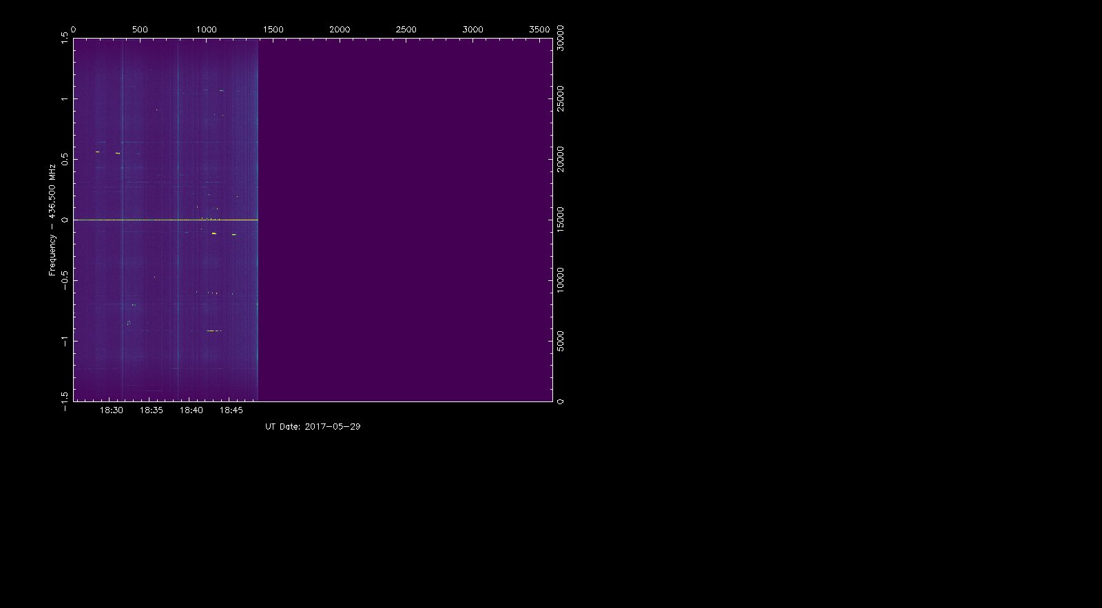
To adjust the waterfall to fill the whole window we can press the r key, obtaining the window below.

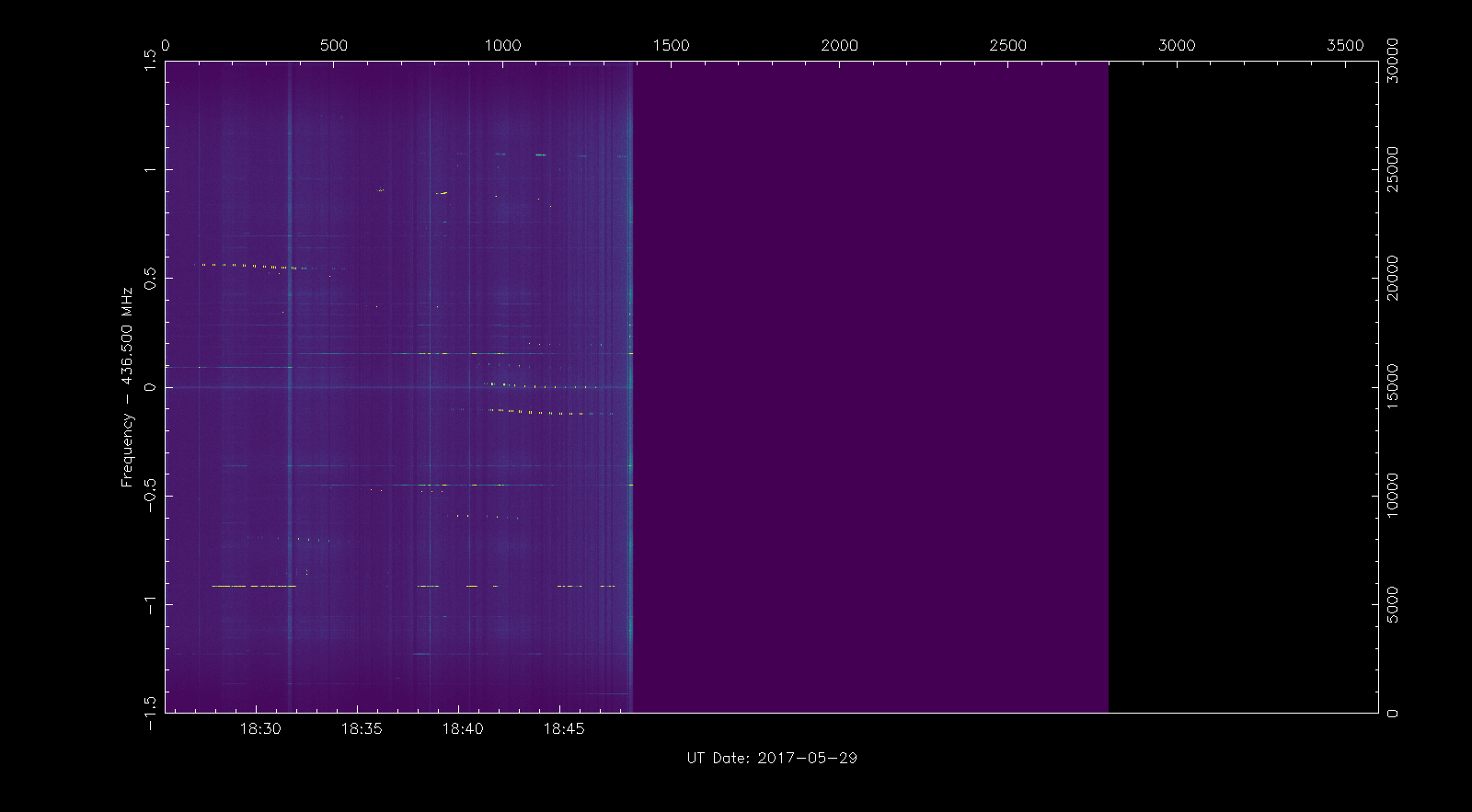
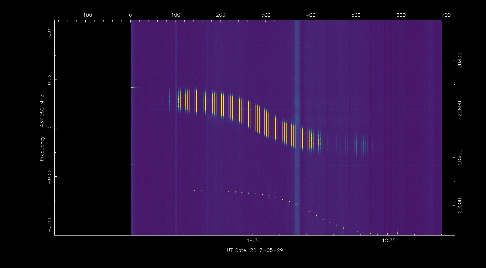
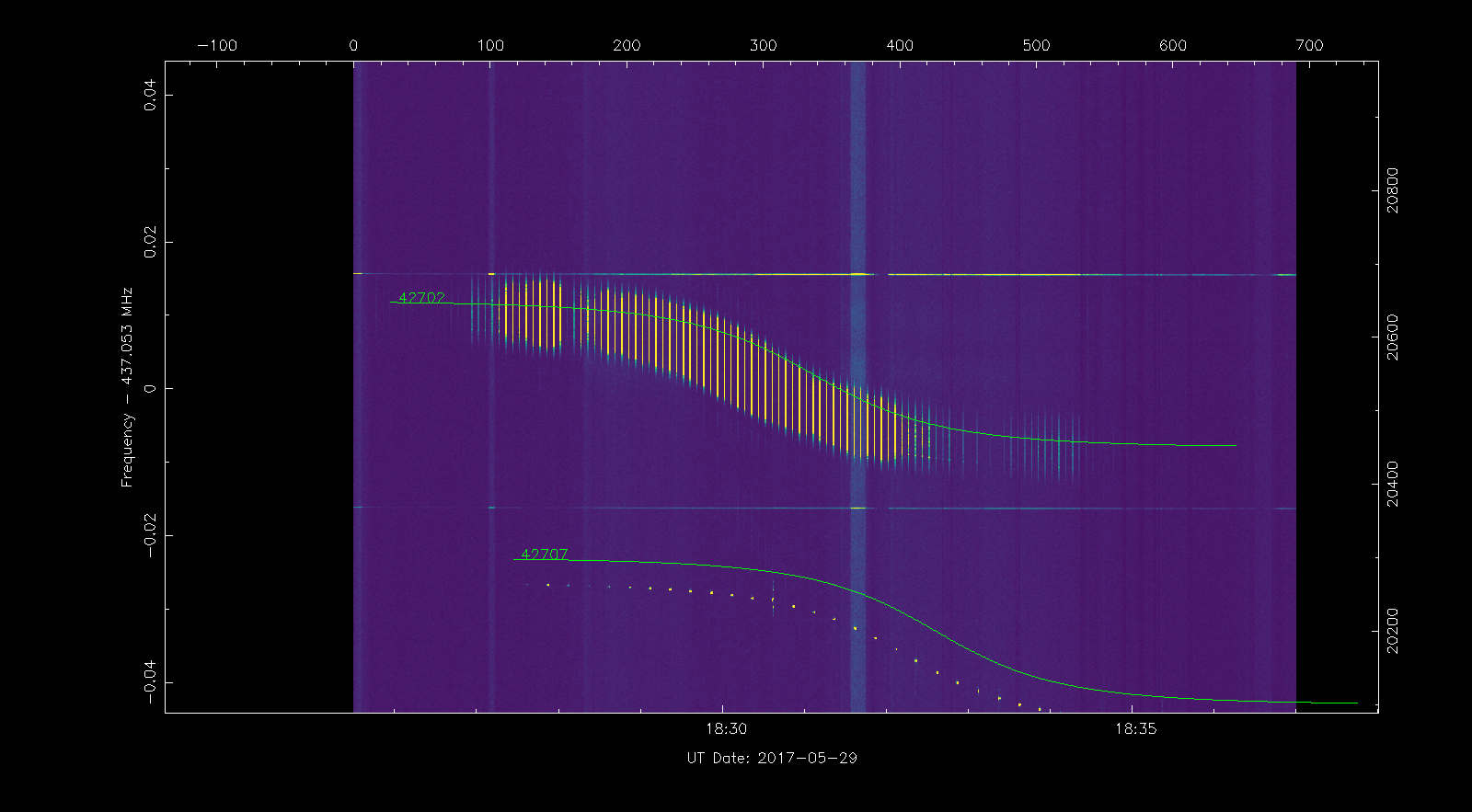
To navigate around the waterfall, we can use the + and - keys to zoom in and out an area around the cursor. The c key can be used to centre the view on the current cursor position, thus moving ourselves. Using these keys we can navigate around and view individual signals. The image below shows the signal of the QB50 satellite US04 Columbia, with its characteristic Doppler curve.

We can use the h to get some help about the commands (key strokes) that can be used within rfplot. The help is printed on the terminal where rfplot was run. This is common with the STRF tools: even though they have a GUI, the interaction with some of the commands is through the terminal (especially when the user needs to type something or an extensive list of information is printed out).

Now you can take some time to familiarise yourself with the different commands that rfplot accepts and to navigate around the waterfall seeing what signals are in the recording. The signal list on the post about the recording can be used as a rough guide.

Exercise 2: plotting Doppler curves on the waterfall

This tutorial explains how to add Doppler curves to the waterfall in rfplot. Displaying the Doppler curves of known satellites is a great aid to identify the signals associated to known satellites and to spot any possible unknown signals in the recording. To plot the Doppler curve of a satellite, rfplot needs to know the orbit of said satellite (which is given in a TLE file), the frequency of the transmitter on the satellite (which is given in a list of frequencies), and the location of the receiving groundstation (which is given in a list of groundstations).

Let us first deal with obtaining the TLEs. These are stored in the directory which has been defined in the environment variable ST_TLEDIR. The default is to read all the TLEs from a file called bulk.tle in that directory. Usually, you would have the latest TLEs stored in that file (there is actually a script called tleupdate in the STRF folder which fetches the latest TLEs from Space-Track) and other sources. However, since we are using a recording from 2017-05-29 we need to use the TLEs from that date.

Actually, getting the TLEs we want is a little tricky. We can’t fetch the TLEs whose epoch is 2017-05-29 (or the ones published in Space-Track on 2017-05-09) because there are many satellites which didn’t have a TLE for that day. What we would like is to have, for each satellite, the latest TLE whose epoch is earlier that 2017-05-29, but there is no way to query the Space-Track database for this.

What we can do is to download a range of dates that guarantees that we have at least a TLE for each object, say from 2017-05-20 to 2017-05-29. Fortunately, STRF scans the TLE file and, for each object, it uses the first TLE that appears in the file, ignoring any other TLEs that might appear later for the same object. Therefore, we can order the file by epoch in descending order to make sure that STRF will always select the latest TLE for each object.

There is a small problem: the result of this query is so large that Space-Track refuses to process it. What we can do is to limit the range of NORAD IDs in the query, say to NORAD IDs greater than 39000, since we know that there are no satellites with a smaller NORAD ID in this recording.

For your convenience, here is the link to submit this query to Space-Track and download the appropriate TLEs. The resulting file is also available in the support gist.

There is another file called classfd.tle inside the TLE directory. This contains the TLEs of classified objects. Since we are not dealing with any classified objects, we will just create an empty file. It is important that this file is present, or otherwise some of the STRF tools will fail.

Now that we the appropriate TLEs, we can add a list of know transmitter frequencies. The list is in data/frequencies.txt in the strf folder. It is simply a list of NORAD IDs and frequencies (given in MHz). For this recording, I have prepared the following file, with the nominal frequencies of each of the Amateur satellites that I know that are present in the recording. The file is also available in the support gist.

42708 435.800
42726 435.900
42714 436.030
42737 436.390
42724 436.420
42725 436.510
42732 436.600
42734 436.705
42701 436.845
42717 436.880
42707 437.020
42702 437.055
42729 437.335
42736 437.370
42721 437.510
42718 437.740
42715 437.400
40927 435.645
40908 437.225
41460 437.425
39090 437.568

Finally, we have to add the location of the receiving groundstation in the file data/sites.txt. This is a list of entries containing the COSPAR number, the ID, the latitude, longitude, elevation in metres and name of each station. I guess that if you don’t have a COSPAR number assigned you can make up your own. This has to match whatever you have set in the ST_COSPAR environment variable. I have added the following entry for my station.

# No ID      Latitude Longitude   Elev   Observer
0000 DE      40.5959   -3.6991    800    EA4GPZ

Once all the files are ready, we can run rfplot as in exercise 1. It will detect the appropriate TLEs and add the corresponding Doppler curves on the screen.

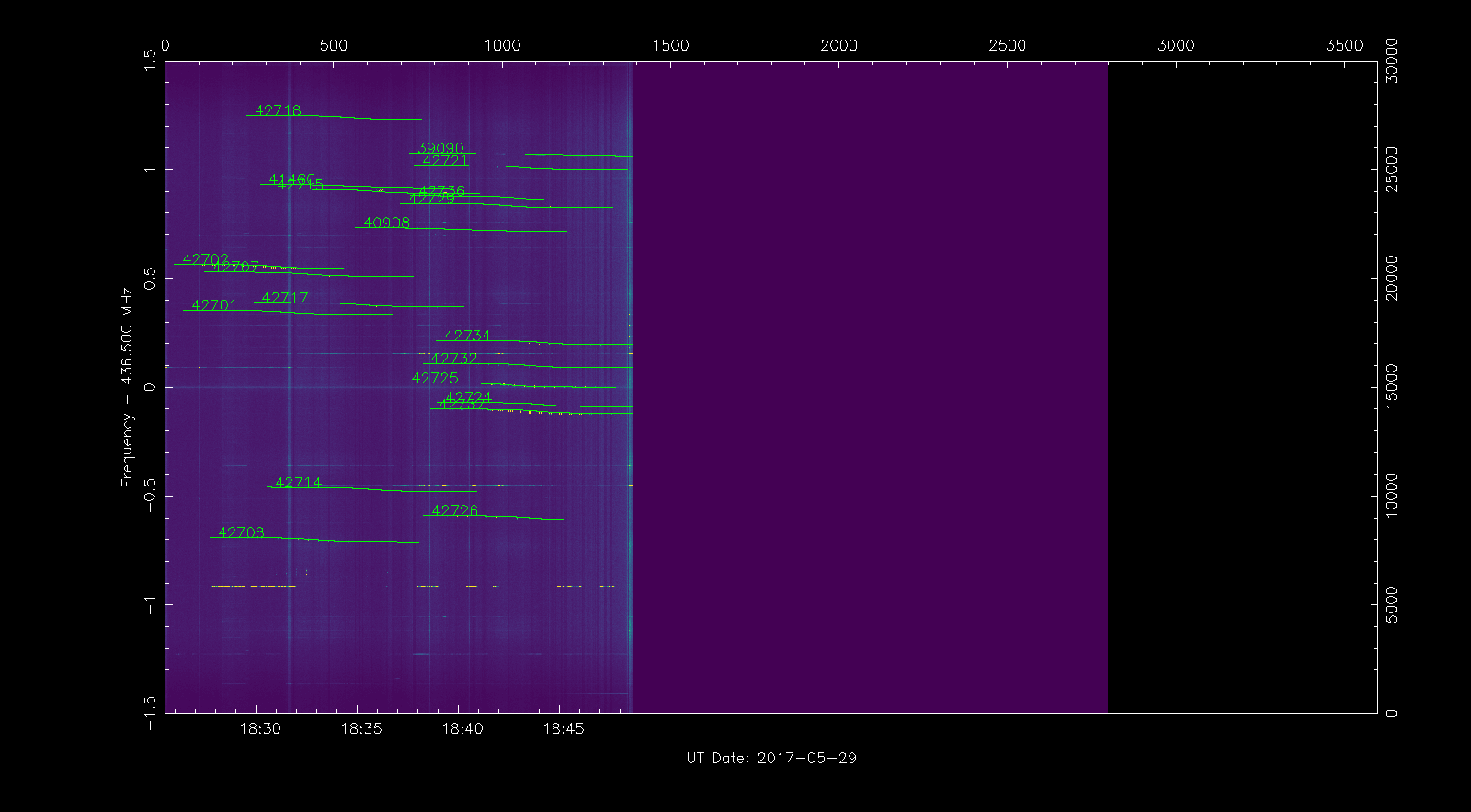
We can zoom in the signal of QB50 US04 Challenger to view its Doppler trace, with NORAD ID 42702. Below it there is another signal which we quickly identify as NORAD ID 42707, or QB50 FR01 X-CubeSat by using its Doppler trace. The display of Doppler traces can be toggled on and off with the p key.

Exercise 3: obtaining Doppler measurements

In this tutorial we will use rfplot to obtain frequency measurements for the signal of one satellite. These frequency measurements can then be used for several things, such as finding a matching TLE to identify the satellite, or refining the Keplerian parameters of a known TLE. Frequency measurements can be generated for any kind of signal that can be identified visually in the rfplot waterfall.

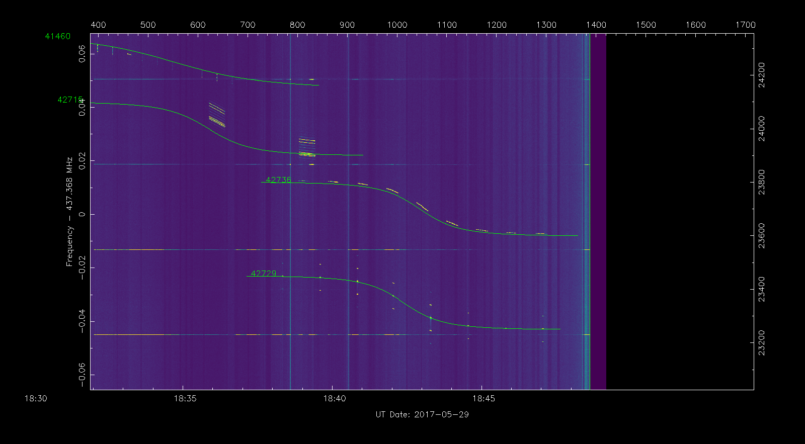
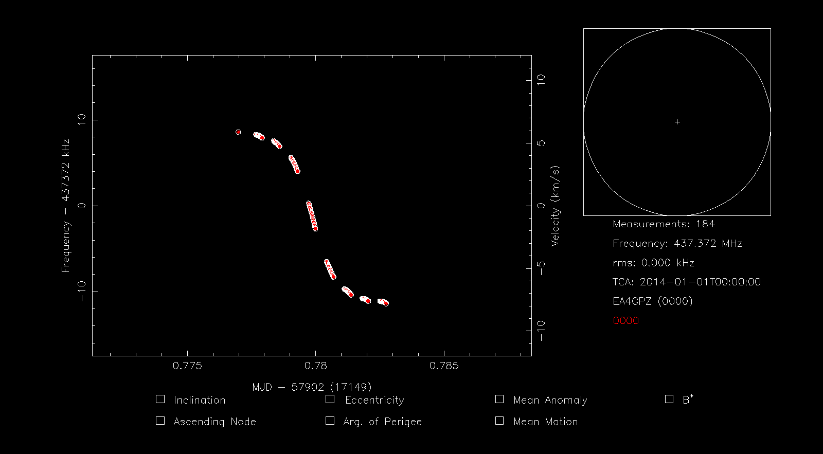
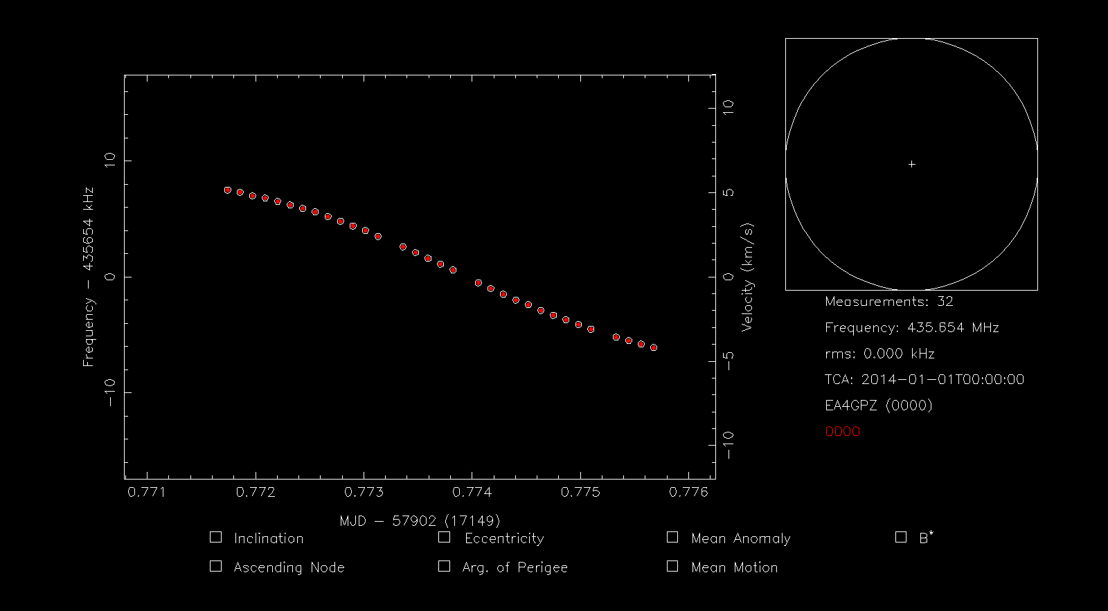
First we navigate the waterfall and find the signal of the satellite QB50 TR01 BeEagleSat, with NORAD ID 42736, obtaining something as in the figure below. This is an ideal signal to obtain Doppler measurements, because it is CW and the duty cycle is relatively high.

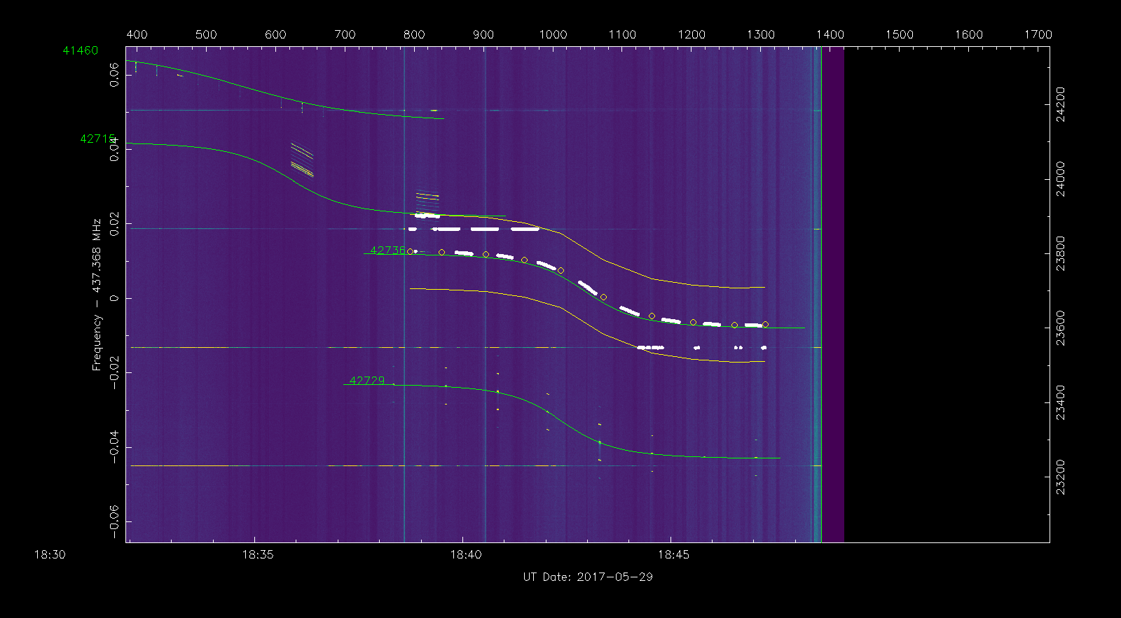
Now we position the cursor over the waterfall at the point where the signal starts being visible and press the s key to add a trackpoint. We move the cursor some distance along the signal and press s again to add a second trackpoint. We continue adding trackpoints at regular intervals along the signal until the point where the signal is lost. These trackpoints define an area from where the frequency measurements will be taken. We should now have something as in the waterfall below.

Now we press the f key to take the frequency measurements in the area we have selected and generate the file out.dat containing these measurements. This is just a list of all the points where a signal (something stronger than the background noise) is present within the area delimited by the trackpoints. The measurement points are shown in white on the waterfall.

As you have probably noted, there are some spurious measurement points that correspond to interference on the waterfall. We will now use rffit to remove these spurious points and obtain a clean measurment. We run

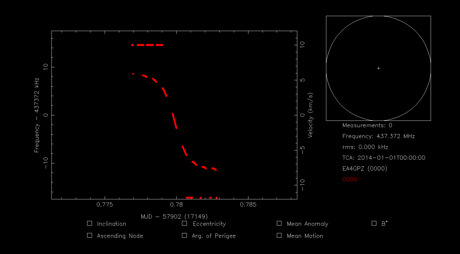
rffit -d out.dat

The figure below shows the rffit window, which plots the measurements contained in out.dat. As in rfplot, we can use r to reset the view and adjust it to the screen.

Now we press the d key to delete points by drawing a box. This allows us to quickly delete the spurious measurement points corresponding to interference, leaving only the points corresponding to the Doppler curve. Next we press s to highlight all the points and then S to save all the highlighted points to a file. The terminal asks us for the filename to use. Here we use 42736.dat. This file is also included in the support gist.

The file we have just created will be used in the next two exercises.

Exercise 4: refining TLE Keplerian parameters

This tutorial shows how to use the Doppler measurements that we have obtained in the previous exercise to refine the Keplerian parameters of the TLE associated with the satellite. In several occasions, such as when there is a release of several objects which are close together, when a satellite is near its decay, when a satellite has manoeuvred, or when the TLEs are too old for any other reason, the accuracy of the TLEs is not very good and they do not fit the measured Doppler curve well. STRF can be used to refine some of the Keplerian parameters to obtain a better match. In this way, we can produce modified TLEs that model the reality better. This introduces the concept of Doppler fitting.

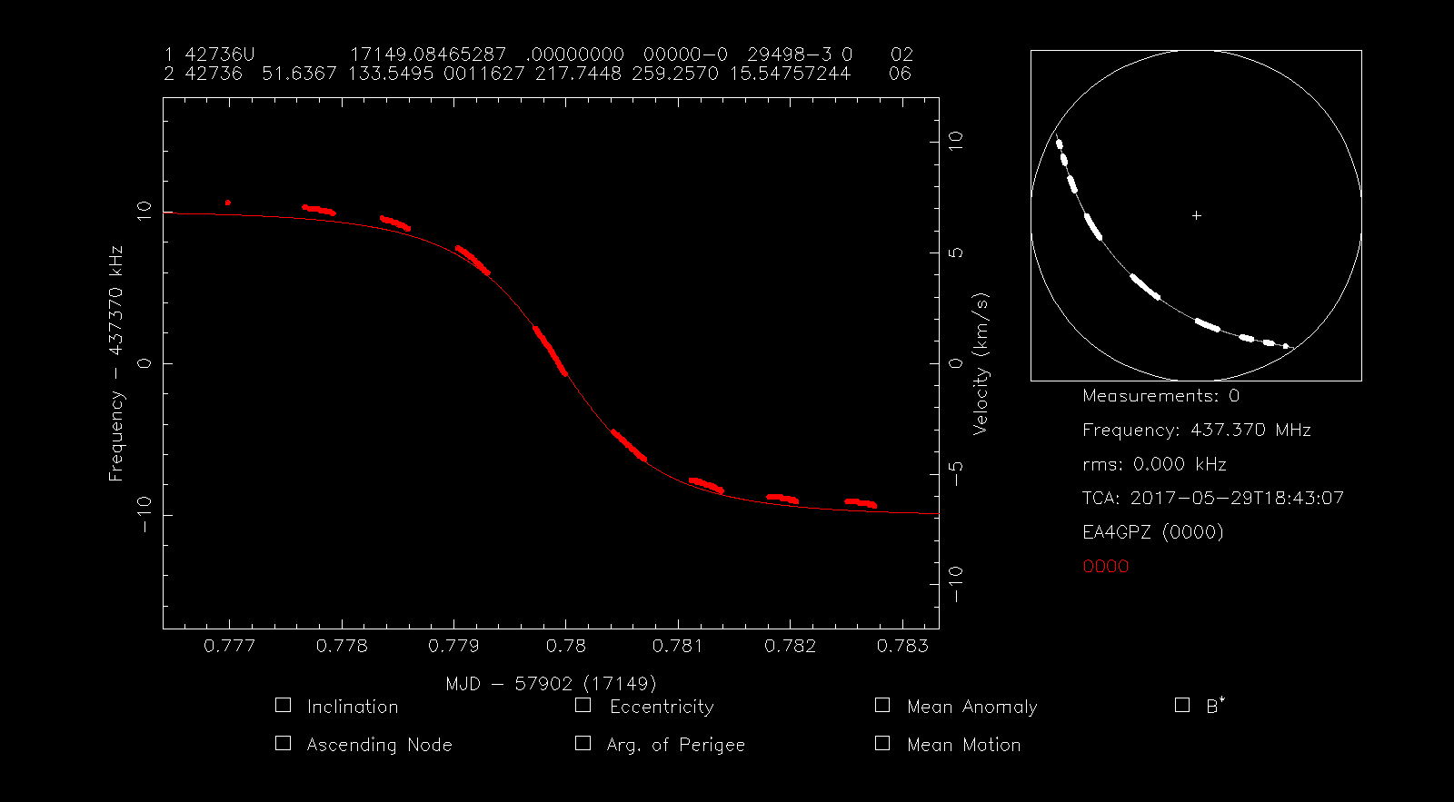
We run rffit as

rffit -i 42736 -c $ST_TLEDIR/bulk.tle -d 42736.dat

to indicate the NORAD ID and TLE file to use for the satellite of study. Since we have indicated the TLE, the Doppler curve is shown and the small graph on the upper right shows the track of the satellite on the celestial sphere and the position of the satellite when the measurements were taken.

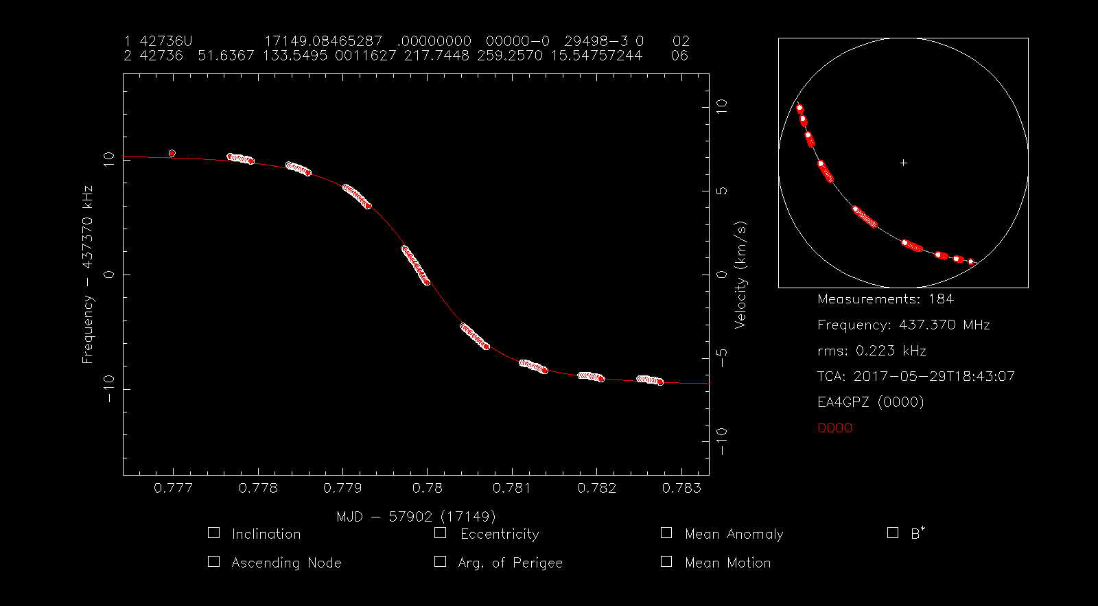
Now we press s to highlight all the points and then f to perform a Doppler fit. Since we haven’t selected yet any Keplerian parameters to modify, this just slides the Doppler curve up and down (corresponding to a fit in transmitter frequency) in order to minimize a least squares problem. This is done because sometimes the transmitter frequency is slightly off from the nominal frequency.

In the figure below we can see that the Doppler curve has moved slightly up in order to fit the measurements better and that the right hand panel now shows an RMS frequency error of 223Hz. The frequency is still shown as 437.370MHz, but this could have changed if the frequency offset had been large.

Perhaps we can find a better Doppler curve by letting STRF vary some of the Keplerian parameters. In this particular case, the satellite we are studying was released from the ISS together with a dozen of other satellites some days before these measurements were performed. Therefore, the different satellites still have not drifted apart much and the quality of the TLEs is not so good, so by varying some of the Keplerian parameters we can try to find a TLE that models the reality better.

If you know anything about orbital dynamics, you’ll probably know that the first parameter we need to optimize is the mean anomaly. This indicates the position of the satellite along its orbit. A change in mean anomaly will simply shift the Doppler curve in time. As small imperfections in the orbit determination (for example, an error in the mean motion) tend to build up an increasing error in mean anomaly, this is the first parameter that is likely to be incorrect when TLEs have drifted or are not good. It is also the easiest parameter to determine well, since even small changes in mean anomaly produce large errors in Doppler near the centre of the pass, as I showed in my post about WSJT-X modes an linear transponder satellites.

Thus we will select the mean anomaly parameter for optimization. You can select several Keplerian parameters for optimization at the same time, but keep in mind that selecting too many will probably give absurd results (which can be spotted because the Doppler curve is still similar but the track on the sky is very different).

We press the 5 key to toggle mean anomaly fitting. Note that the Mean Anomaly checkbox in the lower part on the screen shows a red symbol now. Other numbers could be pressed to select other Keplerian parameters (press h for help). Note that in the figure above we have a TCA (time of closest approach) of 18:43:07. After we perform the fit, this will change according to the change in mean anomaly, and will give us an idea of how much we have shifted the satellite in time along its orbit. Now we press f to perform the fit, obtaining something as in the figure below.

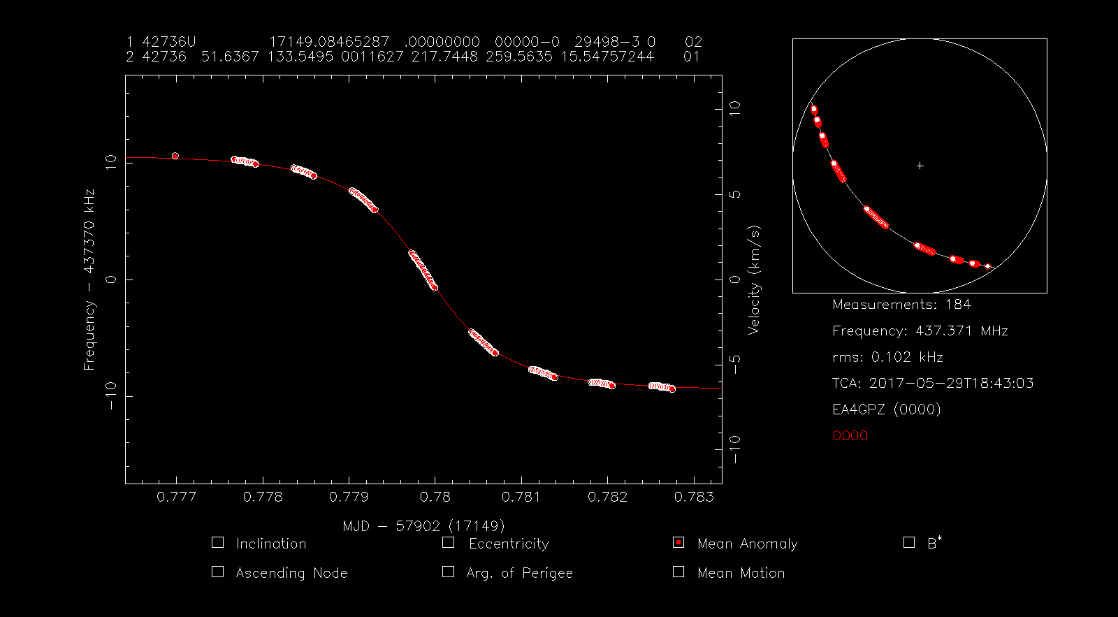
We observe that the TCA has now changed to 18:43:03, so we have shifted the satellite 4 seconds along its orbit (at about 7km/s of LEO orbital speed this is a position error of 28km). Now we have an RMS error of 102Hz, so the fit is much better. The frequency has also changed to 437.371MHz, trying to match better the transmitter frequency. The modified TLE is displayed on the top of the screen.

Since we are happy with our modified TLE and consider it an improvement over the Space-Track TLE, we press w to write the current TLE to a file. The terminal asks us for the name of the file and we choose 43276.tle. This file is provided in the support gist.

Exercise 5: TLE lottery

In this tutorial we simulate a TLE lottery. This is the situation that happens after a launch of several objects. The TLEs corresponding to different objects are still very close together. These need to be assigned to individual satellites transmitting particular signals on different frequencies by means of a Doppler analysis. However, the Doppler curves of many of the objects are very similar and often it is necessary to wait until the objects drift apart more to be able to resolve all the ambiguities.

The recording used in this exercise is ideal to simulate a TLE lottery because it was indeed done during a period of TLE lottery. The only difference with a real TLE lottery is that we know the final outcome, since the individual satellites were identified eventually. Another interesting effect of the TLEs we have downloaded from Space-Track is that some of them are not very accurate (see exercise 4), since the large number of closely spaced satellites makes the tracking of individual objects and the generation of TLEs more difficult. This tends to happen during TLE lotteries.

In this exercise we will use the Doppler measurements for QB50 TR01 BeEagleSat that we have prepared in exercise 3. However, we will pretend that we do not know which is the correct TLE for this object. Even though we now know that the correct NORAD ID is 42736, probably this fact was unknown on 2017-05-29, when the recording was made, and it was determined several days afterwards.

First we run

rffit  -c $ST_TLEDIR/bulk.tle -d 42736.dat 

to load up the Doppler measurements. Note that, in contrast to exercise 4, we are not indicating any NORAD ID to load the TLE, since we don’t know the correct TLE. We are just giving the path to the TLE file.

We press s to highlight all the measurement points, enabling them for Doppler identification. Then we press the i key to perform Doppler identification. The terminal asks us an RMS limit in kHz to filter possible candidates. We enter 0.5, obtaining the following list of candidate TLEs.

42735 0.102 kHz 437.370645 MHz
42735 0.102 kHz 437.370645 MHz
42735 0.096 kHz 437.370631 MHz
42736 0.223 kHz 437.370385 MHz
42736 0.224 kHz 437.370383 MHz
42735 0.096 kHz 437.370631 MHz
42733 0.313 kHz 437.370913 MHz
42733 0.313 kHz 437.370913 MHz
42737 0.324 kHz 437.370269 MHz
42727 0.252 kHz 437.370349 MHz
42734 0.308 kHz 437.370902 MHz
42736 0.105 kHz 437.370565 MHz
42725 0.465 kHz 437.371074 MHz
42728 0.086 kHz 437.370587 MHz
42725 0.383 kHz 437.370986 MHz
42727 0.490 kHz 437.370090 MHz
42736 0.282 kHz 437.370867 MHz
42731 0.115 kHz 437.370677 MHz
42733 0.181 kHz 437.370431 MHz
42728 0.347 kHz 437.370948 MHz
42727 0.304 kHz 437.370292 MHz
42721 0.194 kHz 437.370416 MHz
Identified 22 candidate(s), best fitting satellite is 42728.

This list shows the NORAD ID of the candidate TLEs, the RMS error of the fit, and the precise transmitter frequency given by the fit. Note that the same NORAD ID appears repeated several times in the list, since we have several TLEs for the same object in our TLE file. This wouldn’t happen if our TLE file only contained the latest TLEs for each object, as it would be the case with a real TLE lottery done in the present day. Since our TLE file is ordered by descending epoch, and is scanned in this order by rffit, in general we only concern ourselves with the first time that each NORAD ID appears on the list, as we only consider as valid the latest version of each TLE.

The program tells us that the best candidate is 42728. If we look closely at the list, we see that this TLE has an RMS of only 86Hz. The graphical window loads the best candidate TLE and shows it to us for comparison with the measurements.

Since the TLE doesn’t seem a good fit, we press f to perform a fit in frequency, obtaining the window below.

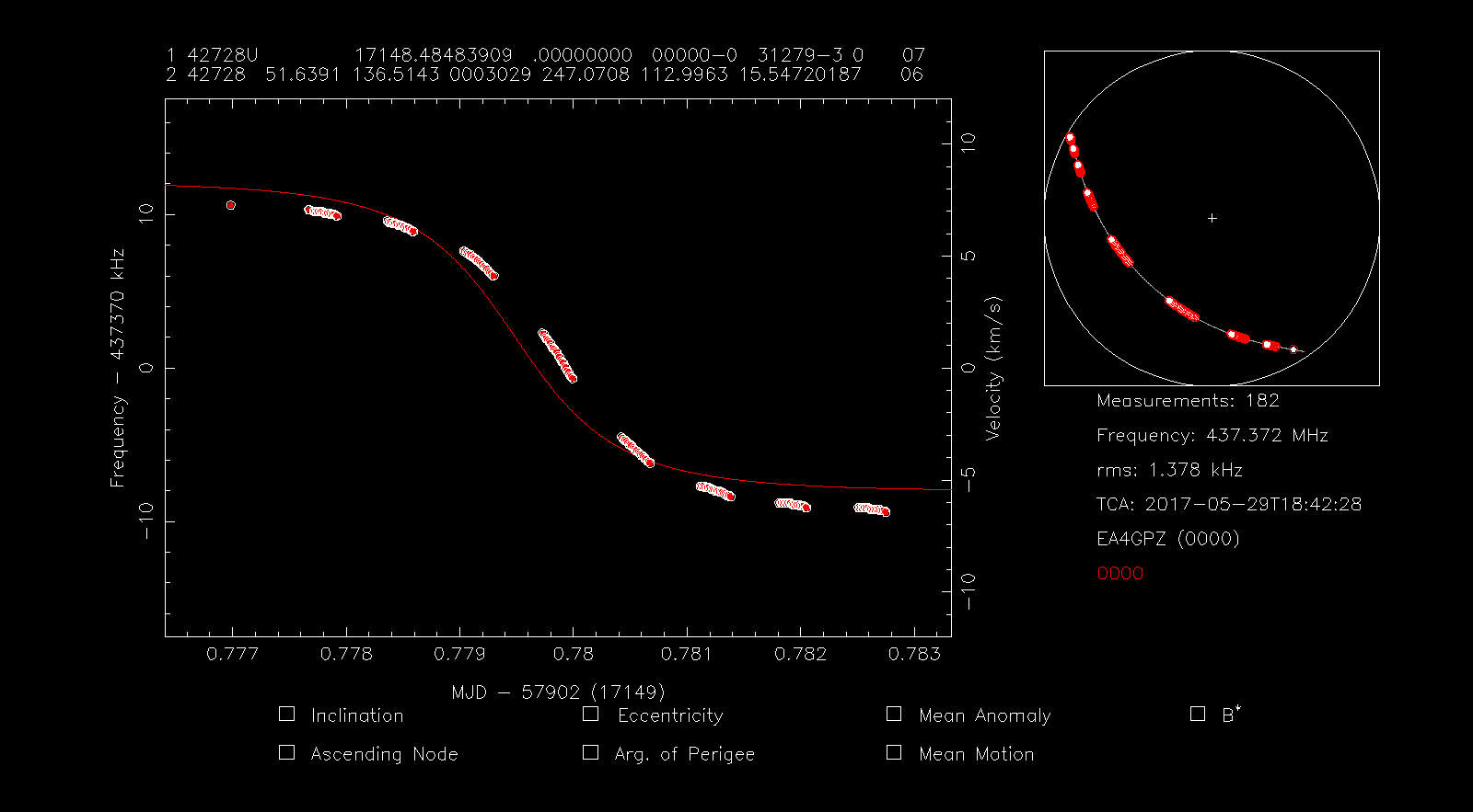
We see that still the TLE is a very bad fit. Indeed the RMS error is 1378Hz, not 86Hz, as the search promised us. Something quite interesting has happened here. Note that the TLE 42728 only appears quite late in the list of candidate TLEs. This means that this best candidate was not the latest version of this TLE. Versions with a later epoch are a much worse fit and do not appear in the list of candidates, since their RMS error is greater than 500Hz. When rffit was told to load up the TLE 42728 for examination, it loaded the latest version of this TLE, since it scans the TLE file until it finds a match. In summary, what has happened here is that the latest version of the TLE 42728 is a very poor match for our signal, but an earlier version was a very good match. We decide to discard this TLE, because we are only concerned with the latest versions of each TLE, as we would normally do in a TLE lottery.

We need to examine the remaining good candidates in the list. If we look closely we see that the only candidates that are worth looking at are 42735 and 42736. Note that 42736 is the TLE we have examined in exercise 4. Thus, we will now load TLE 42735 to compare it against the TLE 43736 that we studied in exercise 4.

We press the g key to get a TLE and enter 42735 in the terminal. The new TLE is loaded. Then we press f to perform a fit, obtaining the window below.

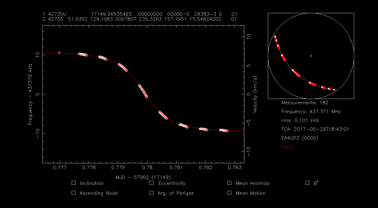
Note that the RMS error is 101Hz, while the RMS error for TLE 42736 was 223Hz. The times of closest approach are 18:43:01 for TLE 42735 and 18:43:07 for TLE 42736. The time difference is only 6 seconds, which translates into a distance of roughly 40km. The two objects are still very close together and we cannot identify the correct TLE until they drift apart more. Indeed, if we had tried to pick up the TLE giving a lowest RMS error we would had made a mistake, as this is 42735 but now we know that the correct TLE is 42736.

Exercise 6: identifying an unknown satellite

This tutorial shows how to identify an unknown satellite by making Doppler measurements of its signal and matching it against the TLE database. The tools and techniques are the same as those used in exercise 5, but here we solve an inverse problem: while in exercise 5 we knew that a signal was associated with one satellite and we tried to find a matching TLE to assign it to this satellite, in this exercise we have knowledge of which TLE is assigned to each satellite and try to find a matching TLE for our unknown signal in order to identify the satellite that transmits it. This is a summary exercise that goes through all the steps explained in the previous exercises.

First we open the waterfall as in exercise 2. If we look attentively at the waterfall, we will find a signal that doesn’t have a Doppler trace. This is because the signal didn’t appear in my post about the recording, because I was unable to decode the signal, as it was too weak. Still, this signal shows a clear Doppler curve, so it must belong to some satellite, rather than being terrestrial interference. We want to identify which satellite is transmitting this signal.

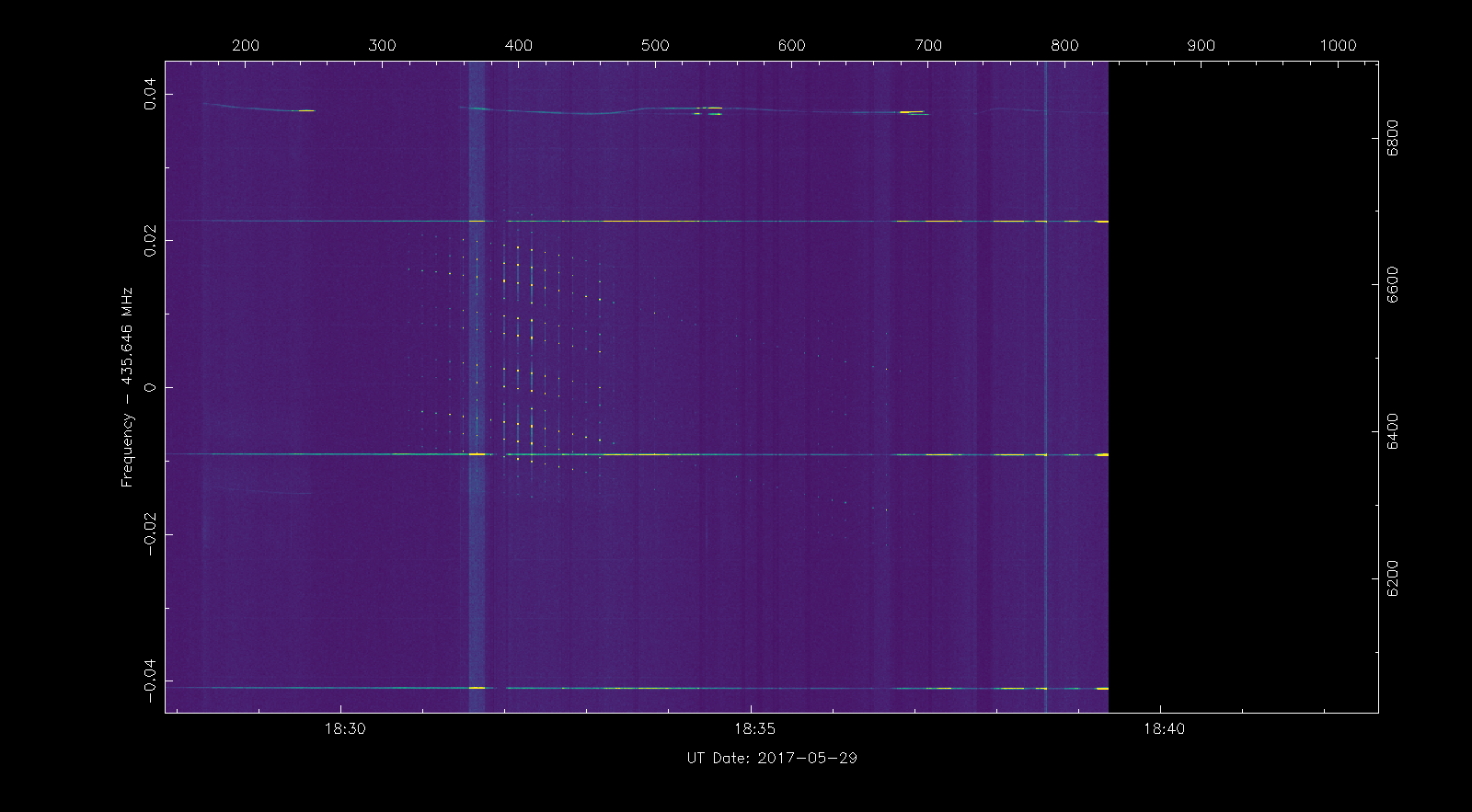
Now we extract the frequency measurements from the waterfall as in exercise 3. Note that since the signal has a complicate spectral shape, we have selected the strongest spectral peak to make the measurements, instead of the signal centre.

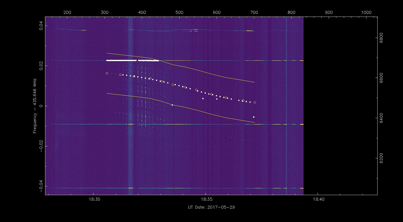
Next we load up our measurements in rffit, delete the spurious measurements and use s to highlight all the remaining measurement points.

Then we press i to identify the signal using the Doppler curve. We use an RMS limit of 100Hz. We see that the best match is the TLE 40928, which corresponds to TW-1A. After pressing f we see that this TLE matches the measurements very well.

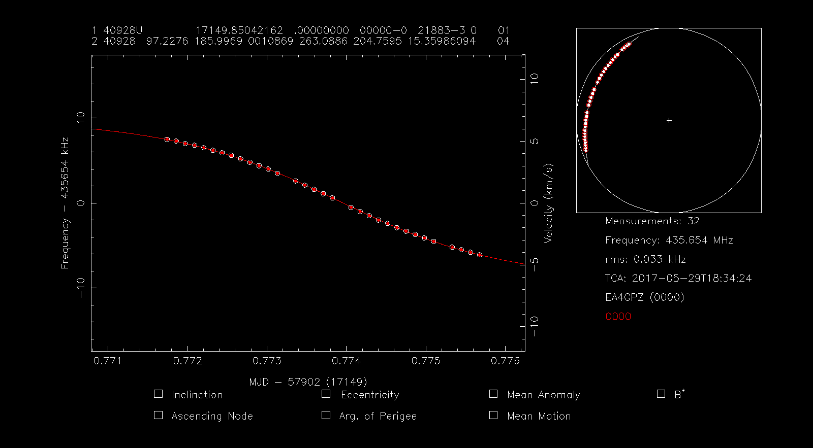
The RMS error is only 33Hz. Finally, to confirm our match, we look at the downlink frequency of TW-1A and see that it has a nominal frequency of 435.645MHz. Since we have performed our measurements at a spectral peak a few kHz above the central frequency, the frequency of 435.654MHz that rffit is showing us is a good match for the nominal frequency. Thus, we conclude that the unidentified signal belongs to TW-1A.