Several weeks ago, in an AMSAT EA informal meeting, Eduardo EA3GHS wondered about the possibility of using WSJT-X modes through linear transponder satellites in low Earth orbit. Of course, computer Doppler correction is a must, but even under the best circumstances we cannot assume a perfect Doppler correction. First, there are errors in the Doppler computation because the TLEs used are always measured at an earlier time and do not reflect exactly the current state of the satellite. This was the aspect that Eduardo was studying. Second, there are also errors because the computer clock is not perfect. Even a 10ms error in the computer clock can produce a noticeable error in the Doppler computation. Also, usually there is a delay between the time that the RF signal reaches the antenna and the time that the Doppler correction is computed for and applied to the signal, especially if using SDR hardware, which can have large buffers for the signal. This delay can be measured and compensated in the Doppler calculation, but this is usually not done.
Here we look at errors of the second kind. We denote by \(D(t)\) the function describing the Doppler frequency, where \(t\) is the time when the signal arrives at the antenna. We assume that the correction is not done using \(D(t)\), but rather \(D(t – \delta)\), where \(\delta\) is a small constant. Thus, a residual Doppler \(D(t)-D(t-\delta)\) is still present in the received signal. We will study this residual Doppler and how tolerant to it are several WSJT-X modes, depending on the value of \(\delta\).
The dependence of Doppler on the age of the TLEs will be studied in a later post, but it is worthy to note that the largest error made by using old TLEs is in the along-track position of the satellite, and that this effect is well modelled by offsetting the Doppler curve in time. This justifies the study of the residual Doppler \(D(t)-D(t-\delta)\).
In this study, we will use the satellite LilacSat-1, which is a member of the QB50 constellation. It was released from the ISS on May 25 this year, and so it is in a circular orbit with an altitude of around 420km and inclination of 52º. The TLE used is
1 42725U 98067ME  17188.90653574  .00007620  00000-0  11662-3 0  9998
2 42725  51.6409 294.7316 0007224  26.7821 333.3542 15.55427837  6725
This was the latest TLE available from Celestrak for LilacSat-1 at the time when this research was started. The epoch is 2017/07/07 19:45:24. We will be looking at the pass starting at 2017/7/9 03:12:00 UTC, which is the next overhead pass at the time when this research started, as seen from my station’s location at 40.6007, -3.7080, 700m ASL. This is how this pass looks like in Gpredict.
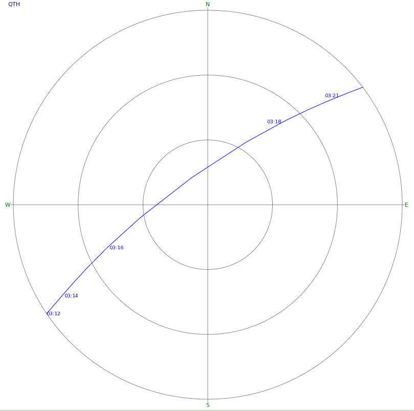
The Doppler, and especially the rate of change of Doppler near the time of closest approach is higher in a high elevation pass, so this overhead pass was chosen to provide a worst case. We will only look at the effect of the Doppler in the downlink of the satellite. This case is interesting if the residual Doppler in the uplink is much smaller than the residual Doppler in the downlink, or if the signal is transmitted by the satellite as a beacon. In the next post we will look at both the uplink and downlink Doppler, as this case is much more involved, since it depends on the geometry between the two stations and the satellite.
The most popular bands used in linear transponder satellites are the 2m band and the 70cm band. Here we will study the 70cm band, since the Doppler is higher. The 2m band is essentially 3 times “easier”. We assume a frequency of 436.5MHz, which is in the middle of the 70cm satellite sub-band (435-438MHz).
We will use PyEphem to perform the Doppler calculations in Python, by calculating the range velocity (change of distance to the satellite with respect to time). It was verified that Gpredict and PyEphem give the same values for the range velocity, as there are some worrying reports that PyEphem computes a wrong range velocity. The Doppler profile for this pass can be seen below.
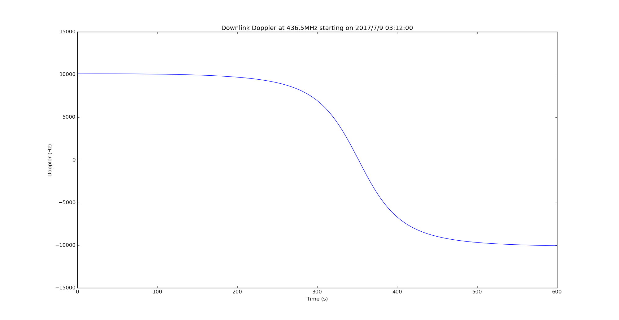
As expected for a low Earth orbit satellite pass on the 70cm band, the Doppler goes down from 10kHz to -10kHz. The most challenging part for Doppler correction is near the time of closest approach, when the Doppler passes through 0Hz, the derivative of the Doppler is largest, and its second derivative changes sign.
Now we turn to the residual Doppler \(D(t) – D(t-\delta)\). Note that this can be approximated by \(-\delta D'(t)\) for small delta. Below we can see the residual Doppler computed for different values of \(\delta\).
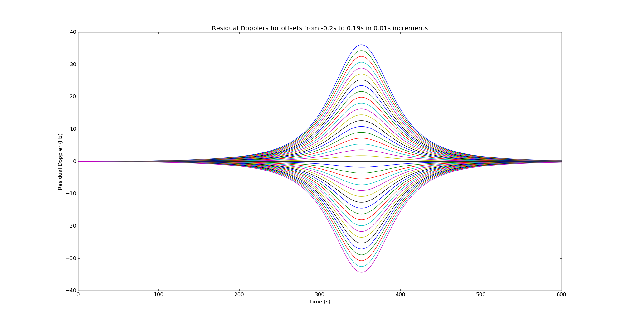
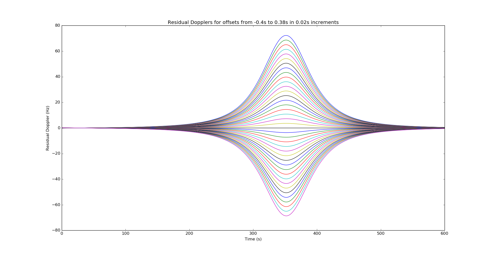
We note that the shape of the residual Doppler is always the shape of the derivative \(D'(t)\). Positive residual Dopplers correspond to the case \(\delta > 0\), since \(D’ < 0\). We also note that even for an offset \(\delta\) as small as 200ms, the residual Doppler is already around 35Hz at the time of closest approach. This can be devastating for many WSJT-X modes, which have tone spacings much smaller than 35Hz. We remark that several WSJT-X modes are able to compensate some form of linear frequency drift. However, near the time of closest approach this is not very helpful. Perhaps much better performance can be achieved by trying to compensate for a frequency drift given by a second order polynomial, but probably this already makes the search space too large.
We see that outside of the interval \(250 \leq t \leq 450\) we can ignore the residual Doppler for the values of \(\delta\) that we are considering here. The residual Doppler is small and more or less linear. This is encouraging: only the 3 central minutes of the pass are challenging. Here we only look at these 3 central minutes, and we decide to start all our WSJT-X signals at \(t = 320\), where the residual Doppler is worst (note that all the modes that will be examined here use periods of 60 seconds, except FT8, which uses periods of 15 seconds).
The decoding tests with WSJT-X have been made with Python. As stated above, PyEphem is used for the Doppler computations, while NumPy is used for DSP computations. The residual Doppler is computed using PyEphem for \(0 \leq t \leq 600\) using a step of 1 millisecond. Then the command line tools from WSJT-X are used to generate WAV files with the signals at a given SNR. These WAV files are read with NumPy, shifted in frequency according to the residual Doppler and stored in disk again. Finally, they are passed to the WSJT-X command line decoder and the number of decodes depending on \(\delta\) is noted. There is more information about generation of sample signals and decoding using the WSJT-X command line tools in this post. The version of WSJT-X used is r8021 from SVN.
The DSP algorithm used to shift in frequency is as follows. A complex sinusoidal oscillator is generated using the residual Doppler frequency. The samples from the WAV file are passed through a Hilbert transform filter and multiplied by the oscillator. Then the real part is taken.
We have studied the following WSJT-X modes:
- JT9A. This is the most sensitive 1 minute mode. It is intended for HF and it is very narrow (15.6Hz, tone spacing 1.736Hz). It is expected that this mode is the worst performer regarding residual Doppler.
- QRA64A. This mode is intended as a replacement for JT65B in EME and also for terrestrial use in VHF, UHF and perhaps the lower microwave bands. The bandwidth is 111.1Hz and tone separation is 1.736Hz. It is designed with Doppler spreading caused by lunar libration in mind. This may help it resist residual Doppler.
- QRA64C. It is the same as QRA64A but with a larger tone spacing, which makes it suitable for EME and some forms of terrestrial propagation in the microwave bands. The bandwidth is 439.2Hz and tone spacing is 6.944Hz. The larger tone separation may help it resist residual Doppler better than QRA64A.
- QRA64E. It is the widest QRA64 mode, with a bandwidth of 1751.7Hz and tone spacing of 6.944Hz.
- FT8. This is a new 15 second mode intended for fast changing conditions such as Es in 6m. It has quickly gained a lot of popularity in HF. It trades off sensitivity by the shorter period. The bandwidth is 50Hz and tone separation is 6.25Hz. The shorter transmit period could help resist residual Doppler, since the total change in Doppler during the period is smaller.
- JT4G. This mode is intended for microwave propagation forms with lots of Doppler spread, such as rain scatter. The bandwidth is 949.4Hz and the tone separation 315Hz. Note that, in contrast to the other modes we are studying, the tone separation of JT4G is much larger than the maximum residual Doppler that we are considering.
More information about these and other WSJT-X modes can be found in Table 3 in the WSJT-X User Guide. It would have been interesting to study JT9H also, which is a very wide variant of JT9A. Unfortunately it seems that there are no command line tools to generate signals of JT9 submodes B through H.
Since the JT9A signal is very narrow and the command line tools support it, to test JT9A we generate a WAV file with 25 JT9A signals at different frequencies. The remaining modes are too wide or the command line tools do not support generation or decoding of multiple signals properly. Thus, 10 separate WAV files with a single signal in each one are generated.
When doing the simulations, we have noted that there is a decoding threshold for the offset \(\delta\). When \(|\delta|\) is greater than this threshold, none or very few decodes are produced. If \(|\delta|\) is smaller than the threshold, then all or almost all of the signals are decoded. The threshold is dependent on the mode, but we have found that it also depends on the SNR of the signals. For a fixed mode, the threshold might be larger for stronger signals.
Thus, we consider three cases for the SNR. First, a low SNR, which is a couple of dBs above the decoding threshold of the mode. Second, -20dB SNR, which is above the decoding threshold for most of the modes studied. Third, -15dB SNR. For an SNR much higher than -15dB, the signals are not weak any more and it may make sense to use other kinds of modes not specialized in weak signals.
The results for the threshold (in seconds) depending on the mode and SNR are summarised in the table below.
| Mode | Low SNR | Low SNR threshold | -20dB threshold | -15dB threshold |
|---|---|---|---|---|
| JT9A | -24 | 0.05 | 0.06 | 0.06 |
| QRA64A | -24 | 0.12 | 0.12 | 0.12 |
| QRA64C | -24 | 0.13 | 0.16 | 0.17 |
| QRA64E | -22 | 0.16 | 0.18 | 0.21 |
| FT8 | -18 | 0.17 | 0.26 | |
| JT4G | -22 | 0.12 | 0.14 | 0.16 |
Note that the low SNR for FT8 is defined as -18dB, since in fact no decodes were obtained at -20dB SNR.
The basic idea of building a WSJT-X decoder that can operate through low Earth orbit linear transponders is to do a search in the offset \(\delta\) until a decode is achieved. In this manner, we try to compensate for the unknown residual Doppler. This will be treated more in depth in a future post. Modes with lower threshold need to have a larger search space, since more values for the offset need to be tried. This increases the computation time.
In view of the table above, we see that JT9A is not a very good idea, since it is not very tolerant of residual Doppler. Surprisingly, JT4G is not a very good performer either if we take into account that its tone spacing is very wide. QRA64E seems a good performer, and its sensitivity is almost as good as QRA64A. Another interesting mode is FT8. Its threshold improves a lot with a better SNR and its 15s period makes it easier to send several messages during a 10 minute pass. Therefore, for the next studies we will centre our attention in QRA64E and FT8. For these modes, it seems that it is acceptable to search for \(\delta\) in steps of 0.2 seconds (perhaps even 0.3 seconds).
Python code. The Python code used in the preparation of this article can be found in this gist.
Acknowledgements. I must thank Eduardo EA3GHS for introducing me to this beautiful and exciting problem and also for his detailed presentation of simulations of Doppler curves using TLEs of different age. His convincing presentation motivated this work.
4 comments