Since I published my Es’hail 2 Doppler measurement experiments, Jean Marc Momple 3B8DU has become interested in performing the same kind of measurements. The good thing about having several stations measuring Doppler simultaneously is that you can perform differential measurements, by subtracting the measurements done at each station. This eliminates all errors due to transmitter drift, since the drift is the same at both stations.
Of course, differential measurements need to be done with distant stations, to ensure different geometry that produces different Doppler curves in each station. Otherwise, the two stations see very similar Doppler curves, and subtracting yields nothing.
The good thing is that Jean Marc is in Mauritius, which, if you look at the map, is on the other side of the satellite compared to my station. The satellite is at 0ºN, 24ºE, my station is at 41ºN, 4ºW, and Jean Marc’s is at 20ºS, 58ºE. This provides a very good geometry for differential measurements.
Some days ago, Jean Marc sent me the measurements he had done on December 22, 23 and 24. This post contains an analysis of these measurements and the measurements I took over the same period, as well as some geometric analysis of Doppler.
It would be interesting if other people in different geographic locations join us and also perform measurements. As I’ll explain below, a station in Eastern Europe or South Africa would complement the measurements done from Spain and Mauritius well. If you want to join the fun, note a couple of things first: The Doppler is very small, around 1ppb (or 10Hz). Therefore, you need to have everything locked to a GPS reference, not only your LNB. Also, the change in Doppler is very slow. The Doppler looks like a sinusoidal curve with a period of one day. To obtain meaningful results, continuous measurements need to be done over a long period. At least 12 hours, and preferably a couple days.
The raw measurements done by Jean Marc can be seen in the figure below. He wasn’t able to record continuously during the three days of measurement, but the characteristic sinusoidal Doppler curve is well visible, meaning that this data is appropriate for further analysis.
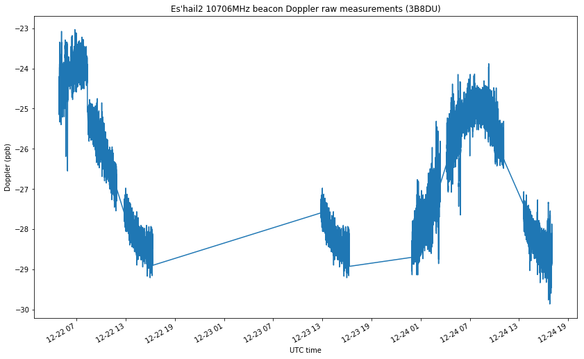
Note the frequency jump that happens around 2018-12-22 08:20 UTC. This is probably caused by Jean Marc’s equipment not being correctly locked in frequency at the start of the measurements. Thus, we will discard the measurements done before this point.
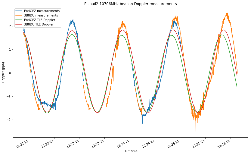
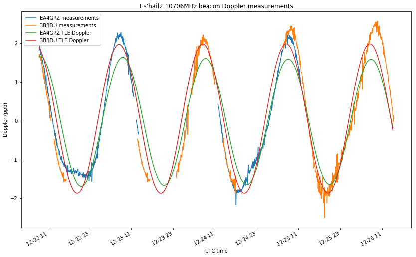
The figure below shows the processed measurements by Jean Marc and myself. I have used averages of 5 minutes and subtracted the mean to remove the transmitter frequency offset.
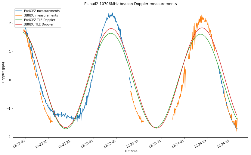
As you can see, I don’t have measurements for a large part of December 23 and 24. During those days I was monitoring the Amateur transponder tests, so I stopped my frequency measurements. Although there is not a lot of temporal overlap between Jean Marc’s measurements and mine, there are still enough measurements to have a good idea of what is happening.
In the figure above I have also included the Doppler predicted by NORAD TLEs (using only one TLE: the one which had the closest epoch). You can see that the Doppler seen by Jean Marc’s station and by my station is very similar. In what follows, I’ll do a geometric analysis to explain why and to show what can be gained by using differential measurements (besides eliminating the transmitter drift). I already did some geometric remarks in my previous post about Es’hail 2 Doppler, so perhaps it’s better to read those first.
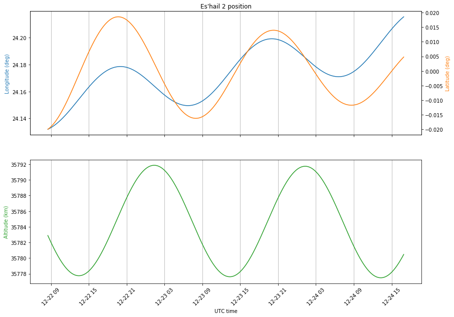
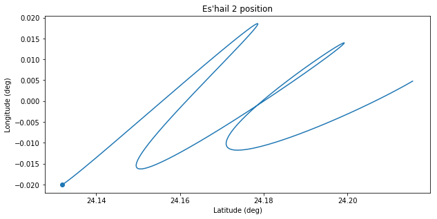
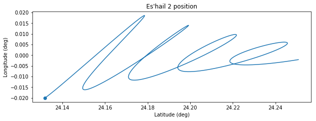
The figure below shows the position of Es’hail 2 during the measurement period in latitude, longitude and altitude coordinates. To compare them, note that an movement of 0.1º in latitude or longitude at geostationary orbit corresponds to 74km approximately. This means that the movement in altitude has an amplitude of 7km, and the movements in latitude and amplitude have an amplitude of 1km.
Besides the amplitude of each of the movements, it is also important how sensitive is the line of sight vector to movements in each of these directions, as I remarked in my previous post. This depends on the projections of each of these directions onto the line of sight vector, which depends on the geometry given by the geographic location of the groundstation.
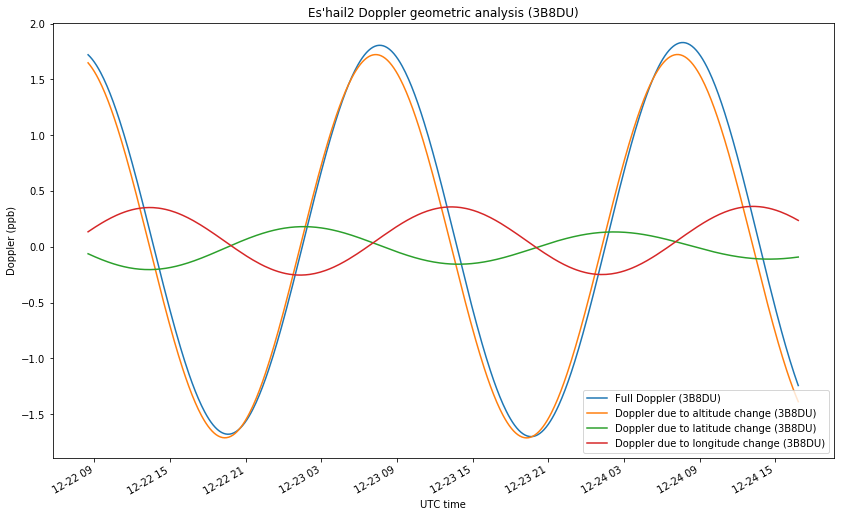
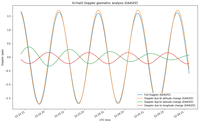
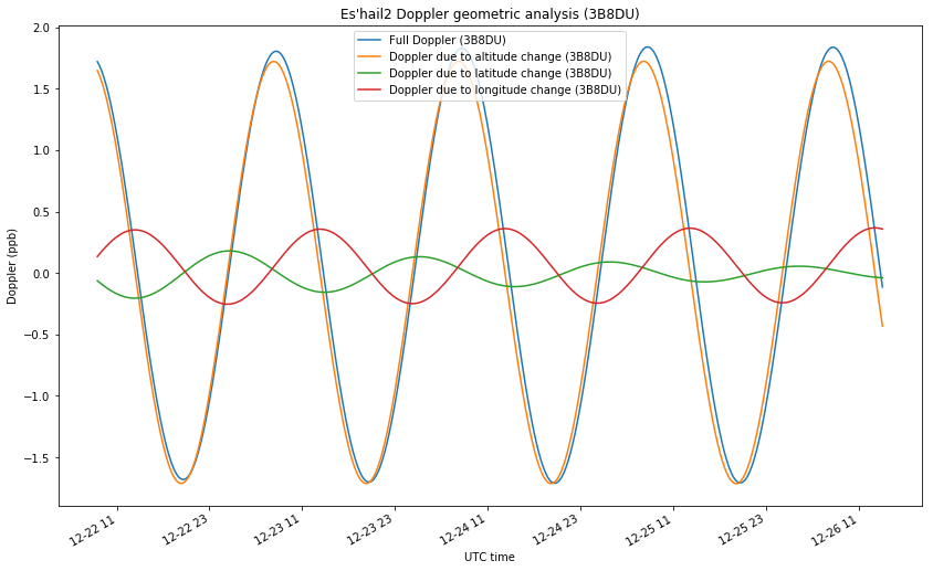
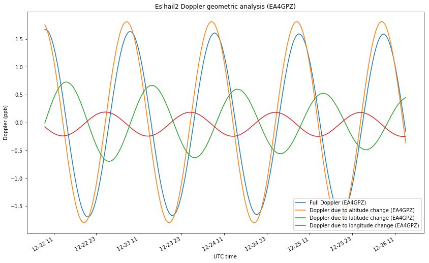
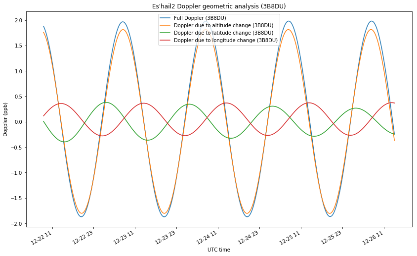
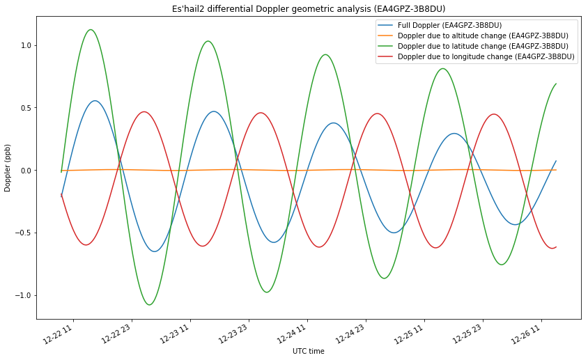
For EA4GPZ, the projections for altitude, latitude and longitude are respectively 0.992, -0.108 and 0.059. For 3B8DU, they are 0.994, 0.059 and -0.088. With this data, we can plot the amount of Doppler that is caused by the movements in each of the directions, so that the total Doppler is the sum of three components. This is shown in the two figures below.
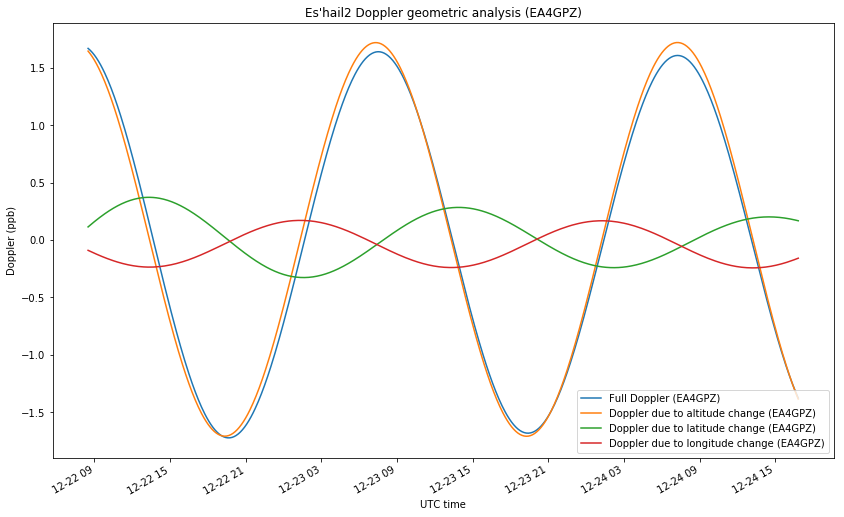
For the geometry of EA4GPZ, we see that most of the Doppler is due to altitude changes, while the movements in latitude and longitude contribute in small equal magnitudes.
The situation for 3B8DU is very similar, except that the signs of the Doppler due to latitude and longitude changes are opposite, due to the two stations been located on opposite sides of the satellite.
As we have seen, both stations have a sensitivity to altitude movements close to one. This is indeed the case for all the stations on the surface of Earth, due to the fact that the geostationary radius is much larger than the Earth radius. This means that the Doppler due to altitude changes will be very similar in all stations. By subtracting, we can eliminate most of the contributions of this component and study the contributions from latitude and longitude changes.
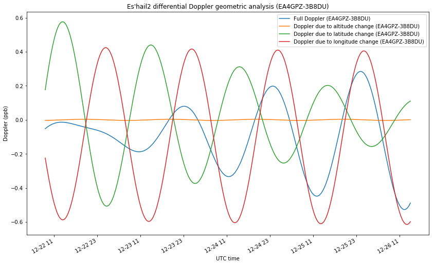
The figure below shows the geometry of the differential Doppler between EA4GPZ and 3B8DU. As we expected, most of the contribution of altitude changes is eliminated. The contributions of latitude and longitude changes result approximately opposite, so the final full Doppler is something small.
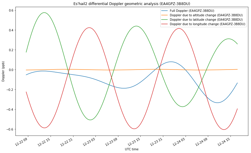
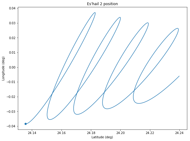
The reason for this is that the differential Doppler between EA4GPZ and 3B8DU is sensitive to movements in the northwest-southeast direction, while the satellite was moving on a northeast-southwest direction, as the figure below shows (the dot indicates the position at the start of the measurement interval). Thus, a station located in Eastern Europe or South Africa would complement well the geometry of EA4GPZ and 3B8DU by giving sensitivity in the northeast-southwest direction.
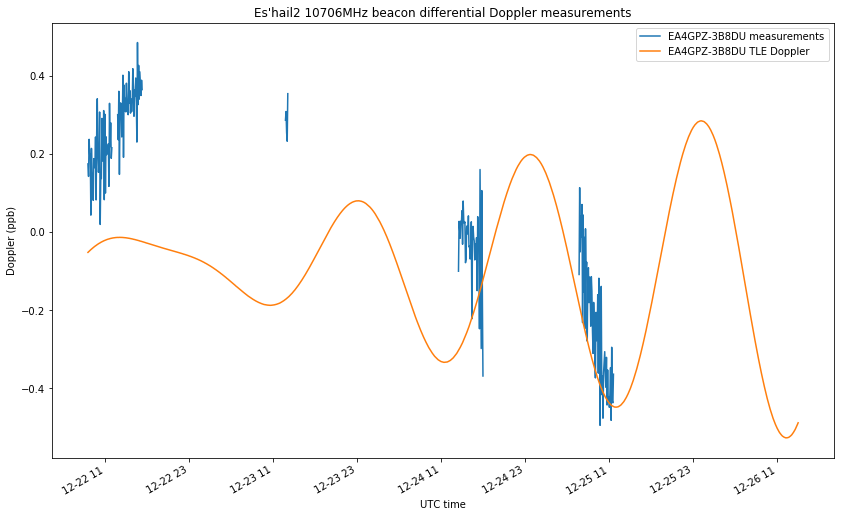
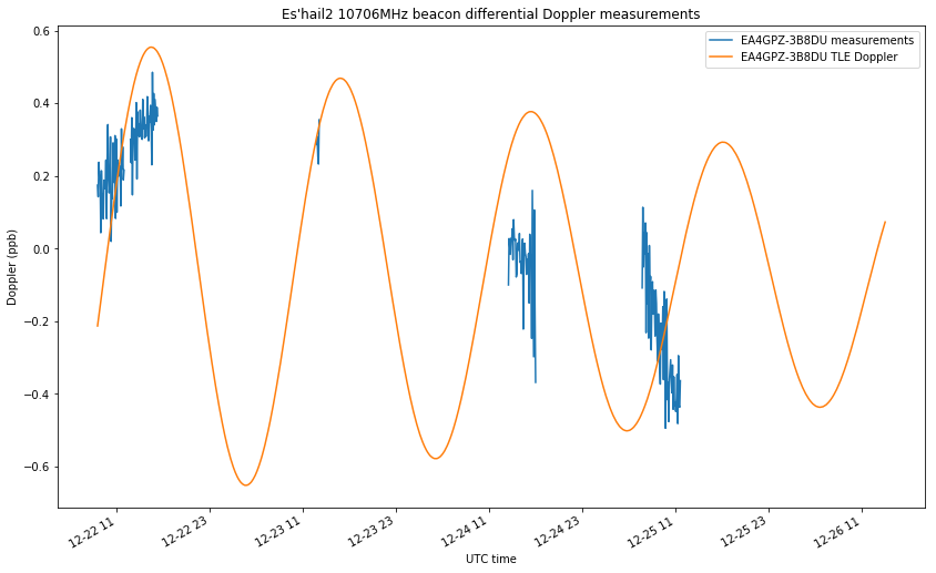
The differential Doppler measurements between EA4GPZ and 3B8DU are shown in the figure below. As remarked above, simultaneous measurements with both stations are only available for small periods of time, unfortunately.
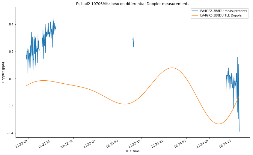
Still, we see that the available measurements don’t match the predictions by the TLE. Since the experimental setup is very precise (everything is GPDSO locked, we are performing differential measurements to eliminate transmitter frequency offset, and the rate of change of Doppler is very slow, so precise time-tagging of measurements is not critical), this clearly indicates an error in the TLEs. Thus, we are improving upon the TLEs with our Amateur orbit determination system.
Note that, as shown in the figure above, Es’hail 2 main movement was along a northeast-southwest line, and our measurement setup is sensitive to movements orthogonal to that line. This means that we’re measuring small deviations from the dominating trend in latitude-longitude movement (which is caused by the inclination, the RAAN and the argument of perigee). These small deviations are very sensitive to the Keplerian parameters and orbital perturbations, so it is not very surprising that the TLEs don’t match well our differential measurements.
It would be very interesting to continue these differential measurements over a window of a couple of days, and adding a third station that provides sensitivity to the northeast-southwest direction.
The calculations in this post have been done in this Jupyter notebook.
Update 2018-12-31: I have just noticed that I had another set of measurements from Jean Marc. The complete set of measurements can be seen below.
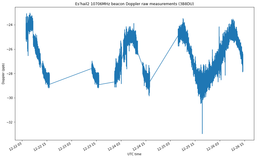
I have redone all the plots above including these measurements.
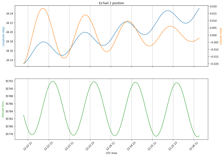
Also, to show how sensitive is the differential Doppler to small changes in the TLEs, I have redone all the calculations using the nearest TLE to 2018-12-24 (the above plots use the nearest TLE to 2018-12-23). Note that the behaviour of the satellite position in latitude and longitude is rather different.
Hello Daniel,
can you please tell me if it is possible for you to find out, what frequency fluctuation there is when you are measuring every 10 seconds ( or 5 seconds if possible ) with the help of EsHail2 10,706 GHz beacon ? It is very important for VARA SAT transmissions. If the frequency fluctuation in such a short time period is to high, the higher speed levels of VARA SAT can not be achieved. It is no problem at all for VARA SAT to handle a long period of time (24h) frequency fluctuation of +/-20 Hz.
73
Bernd, DL2BZ
Dear Bernd,
The VARA modem is closed source software without any available specifications, so I won’t support or encourage its use in Amateur radio.
As you can see in the plots above, when not doing any filtering (so the measurement interval is around 3 seconds), the measurement noise is around 1ppb or so. However, I don’t know what this has to do with transmitting VARA through the QO-100 transponder.
Hello Daniel,
under https://rosmodem.wordpress.com/ you can download the
VARA HF Modem Specification
Revision 2.0.0 April 5, 2018
Jose Alberto Nieto Ros, EA5HVK
In chapter 3.2 Jose declares:
Frequency stability. The short term frequency stability of the transmitter and receiver shall be less than 0.5 Hz/second for SSB operation. I will sent the document to you via email.
I hope that you understand now, why the frequency drift in a time period of 5 seconds is very important for reaching the higher speed levels. Can you please tell me, if you can verify with your doppler measurements @ QO-100 what frequency fluctuations there are in a time period of 5 to 10 seconds ?
By the way: The fastest VARA transmission via QO-100 was 18140 bytes/min:
https://forum.amsat-dl.org/index.php?thread/2829-is0grb-winlink-server-on-qo-100-dial-10489635-0-usb/&postID=11441#post11441
73
Bernd, DL2BZ
Hi Bernd,
I don’t find anything called “specifications” in rosmodem.wordpress.com. I’ve taken a look at the PDF files you sent me by email and these are by no means enough for someone to be able to build their own VARA decoder (or transmitter). Additionally, in the VARA HF Modem Specification 2.0.0 it clearly says that “VARA HF Modem is a propietary system developed by Jose Alberto Nieto Ros EA5HVK and can be used under shareware license.” So I maintain my claim that VARA is closed source software without any available specifications, so in my opinion it has no place in Amateur bands (of course this is just my opinion, not the Regulations, so anyone can use it if they want to).
Also, using an OFDM modem over a geostationary satellite is not a good idea. You don’t have any multipath, so OFDM brings no advantages and it gives all the problems with frequency stability you’re seeing. The good idea is to use a single-carrier PSK modem. Just look at DVB-S (-S2, -S2X also).
A transmission of 18140 bytes/minute (which works out to 2419bps) is not at all surprising. I have pushed 2kbaud 8PSK through the narrowband transponder (staying at the same power as the digital beacon) with few bit errors. This gives a rate of 6000bps. With some light 9/10 FEC, a net data rate of 5600bps shouldn’t be difficult to achieve.
About the frequency stability, 0.5Hz/second is not a precise measure of anything. It should be interpreted as a rule of thumb. Usually, when someone gives this kind of figure, what he means if that in the very simple theoretical case when the system is subject to a linear frequency drift, then something about the receiver (coherent integration, PLL loops, etc) breaks for a drift larger than 0.5Hz/s. It doesn’t say anything about the behaviour of the system in complex real world situations, and it doesn’t say that the system will behave correctly as long as the frequency drift is always kept under 0.5Hz/s (interpret this however you will, as a derivative or as a finite difference).
Of course the question “what frequency fluctuations are there in a time period of 5 to 10 seconds?”, when asked as such, doesn’t have a definitive answer, since it is just a vague question and not a formal one. Additionally, whatever may be some kind of answer to this question, it won’t have much to do with the 0.5Hz/s figure we spoke about.
There are several formal measures of frequency stability (it is actually an interesting topic tied to phase noise and such). One of the most popular is Allan deviation. So you could phrase a question in terms of Allan deviation.
Of course, if you know anything about Allan deviation, you’ll know that the deviation at a particular observation time (it is usually written “tau”) doesn’t have anything to do with the deviation at other values of tau. This is the reason why I stress that your idea to measure “fluctuations” in a period of 5 to 10 seconds doesn’t have much to do with the 0.5Hz/s figure. And also the reason why 0.5Hz/s doesn’t really mean anything in the real world, where frequency drift is a stochastic process instead of a linear ramp.
Coming back to the 0.5Hz/s thing, maybe this could be phrased in terms of Allan deviation as a deviation of 5*10^(-11) at tau = 1s (assume a carrier frequency of 10GHz). Now, a TCXO has an Allan deviation on the order of 10^(-9) for tau = 1s. The fact that you are able to use VARA over QO-100 using TCXOs says that this 0.5Hz/s figure should be taken, at best, with some care.
I have all my QO-100 groundstation locked to GPS using a DF9NP GSPDO (which has VCTCXO disiplined by a uBlox LEA-4S with a PLL). This means I could measure the Allan deviation of the QO-100 transponder local oscillator against my GPSDO. I expect that the QO-100 LO is probably more stable than my GPSDO for small tau’s, so a better frequency reference would be needed for meaningful measurements at small tau’s.
All this would be quite interesting as a scientific experiment, but I fail to see what this has to do with you people using VARA over the transponder. Unless you’re all running locked to GPS, most likely the frequency stability of your groundstations is worse than that of the QO-100 LO.
Hello Daniel,
you pushed 2kbaud 8PSK through the narrowband transponder.
I ask myself, how did you do this ?
I only can find a 1200 baud 8PSK modem in fldigi.
This leads me to the question, how you managed to use a 2kbaud 8PSK modem ?
Which software or firmware did you use ? Which hardware ? Which operating system ?
I’m shure that the QO-100 LO is using a rubidium reference which is about 1 exp -15 in Allan deviation. I use a reference about 1 exp -11: Thus using a 10.5 GHz Signal the frequency fluctuation is max. 0.5 Hz and not +/- 3 Hz in a time period of 5 seconds.
I’m afraid, that there are three other factors to take care:
1. TEC ( Total Electron Content )
2. Mechanical instability/movements of the QO-100 satellit ( not really exactly GEO stationary )
3. Ionospheric scintilations ( causes signal interferences )
Do you know this URL ?
https://www.sws.bom.gov.au/Satellite
There you can read:
“Total Electron Content (TEC) is a measure of the total number of electrons in a vertical column of the ionosphere. It is indicative of the average electron density of the ionosphere and is proportional to the delay in transmission of radio frequency signals (such as GPS) through the ionosphere. When there is increased ionisation in the ionosphere caused by enhanced solar radiation or geomagnetic storm conditions, particularly during times of enhanced solar activity, TEC may increase significantly, often in an spatially non- uniform way. This has implications for GPS navigation and satellite communications as well as HF radio communications.”
I’m understanding the term “delay in transmission of radio frequency signals” that way, that there is a frequency fluctuation/drift because of TEC !
I would be glad if you can find out with your doppler measurement setup, how big the frequency fluctuation is on the 10.5 GHz @ QO-100 beacon-signal in a time period of 5 to 10 seconds. Of course it would be necessary to make measurements each day in a period of a month, I suppose, in order to find out, if there is a correlation to the daily changing TEC conditions.
Not only VARA SAT communications is suffering because of the frequency fluctuation but also Pactor4 protocol, which is often used for emergency communication.
The aim for me is to achieve ultra-stable digital communication on QO-100 for the use with the “winlink global radio email-network”.
I’m very glad that IS0RGB ( Roberto ) has established the first VARA SAT winlink email gateway:
“Geostationary SAT QO-100 on 26 Est. Dial RX Downlink 10489.635 MHz USB. Dial TX Uplink 2400.135 MHz USB”.
I’m still missing Pactor4 winlink email gateways on the QO-100 NB transponder…
The faster and more stable the communication protocol and it’s used hardware is, the more efficient the channels can be used.
73
Bernd, DL2BZ
Hi Bernd,
The 2kbaud 8PSK transmissions were done with GNU Radio. I haven’t published a post yet, since this is still a work in progress, but you can see some tweets. The hardware was my usual QO-100 groundstation.
Rubidium is by no means 10^(-11) ADEV. See here, for example. Even Galileo clocks are worse than 10^(-15). 10^(-15) is a state of the art active Hydrogen maser or something like that.
I don’t agree that the ionospheric delay or the movement of the satellite are important. They are very slow changing factors.
Scintillation might play a role (note I said “might” just not to rule its existence out completely), but it is an uncommon phenomenon best studied at L-band (since it affects GNSS signals). I don’t know how strong or common it is at 2.4GHz (certainly less that at L-band) and I expect that it should be negligible at 10GHz.
Bernd,
As explained by Daniel, Vara, Pactor etc… have been designed for HF (I am running a Winlink HF station for over 5 years and well acquainted with these). I also agree with Daniel’s points as using QO-100 on both the NB and WB transponders (up to 4MS DVB-S2) Over QO-100 no need of these.
You may use the WB transponder for high speed data experiment also with minimal error correction a the bird signal is good both on uplink and downlink.
As regards Winlink, it is mostly used by offshore seafarers (like me) and having a dish for GEO at sea is not really practical (at least for most) HF is the more appropriate.
As regards EMCOM QO-100 is surely a great asset, but data transfer may be enhanced with a mode such as PSK or other which are much more efficient on data transfer particularly on the WB transponder.
My one cent input.
Jean Marc (3B8DU)
Hello Daniel,
yes you’re right, because
https://en.wikipedia.org/wiki/Atomic_clock
tells us, that the Allan deviation of Cs = 1 exp -13, Rb = 1 exp -12, H = 1 exp -15 and Sr = 1 exp -17.
Thus I’m saying, that the QO-100 LO has a H-atomic clock with Allan deviation of H = 1 exp -15. Thus the LO of QO-100 is not responsible of the frequency fluctuations of +/- 3 Hz in a time period of 5 to 10 seconds.
If your thesis is correct, that the frequency fluctuations are not caused by ionospheric TEC delay, movement of the satellite and scintillation, I’m wondering, where they come from finally ? I have no clue about that. I made about 100 transmissions of a 100 kbytes file, while observing the whole SDR spectrum of the Narrow Band transponder of QO-100. Each time the transmission speed is reduced from 3500 to 2000 baud I can watch clearly uncommon interferences on the whole spectrum of the transponder. When the uncommon interferences disappear, the speed is increasing up to 3500 baud again.
I’m using the URL https://eshail.batc.org.uk/nb/ in this context.
If you take a look at this short video, you can easily see, that there are indeed relevant frequency fluctuations.
https://www.youtube.com/watch?v=X6wByqUONyk
I decoded the beacon on my own with my DL2BZ transverter setup ( not using the https://eshail.batc.org.uk/nb/ ) with the result, that it correlates with the video.
73
Bernd, DL2BZ
Hi Bernd,
Let’s keep this simple. The local oscillator on the QO-100 doesn’t have an Allan deviation of 10^(-15) for any tau. Most likely it has a deviation on the order of 10^(-10) or at best 10^(-11) for tau on the order of 1s to 100s. Specific details haven’t been published but could be measured by someone with a groundstation locked to a good frequency reference.
The short term frequency variations you are seeing are due to your transmitter and receiver (to a larger or smaller extent, depending on whether you use a TCXO or a good OCXO) and to the transponder LO. Keep in mind that 3Hz at 10GHz is 3*10^(-10), which is pretty good stability for an Amateur station. There is no other significant effect.
Hi Daniel,
I’m using this 100 EURO device:
Connor-Winfield OH300-50503CV-025.0M bought from digikey.
Short Term Allan Deviation (1s) Fo = 10 MHz: 1.0E-11.
I already made a long burn in process to the VCOCXO – Thus the frequency drift should be not higher than 0.1 Hz @ 10 GHz.
The satellite is 70 Million USD + 60 Million USD shipping to GEO.
I really can’t imagine, that the LO of QO-100 is not stable enough… – but it’s true , we don’t know !
Of course the frequency deviation of +/- 3 Hz can come from the VCOCXO or the PLL of the LNB or the PLL’s of the DL2BZ transverter. It does not come from the SSB-Transceiver, because I verified this already.
I’m not able to make precise doppler measurements and I don’t know who can do this ?
73
Bernd, DL2BZ
Hi Bernd, is all your system (LNB, transverter, transceiver, PC soundcard if you use one) locked to this OCXO? If so, you can do precise frequency measurements through the QO-100 transponder.
To measure the QO-100 transponder LO, put up a CW carrier through the transponder and measure its downlink frequency using WSJT-X. Then use the Python code in this post to compute Allan deviation. It’s not difficult at all.
If possible, also make a WAV or IQ recording to measure short term (tau < 1s) Allan deviation or phase noise.
Hi Daniel,
LNB and transverter is locked to the same VCOCXO. The transceiver has a transceiver-built in soundcard which is connected to the PC ( coffee lake, with Windows 7 ). The transceiver works in 10m Band and has a 0.5ppm Tcxo. Thus I’m afraid, that a measurement measures the sum of the following drifts (without mentioning the drift of the VCOCXO which must be added of course):
1. Drift of the transceiver built in soundcard
2. Drift of the 0.5ppm transceiver-Tcxo
3. Drifts of the PLL’s of the DL2BZ transverter ( Rx- and Tx-paths )
4. Drifts because of ( TEC, scintillation, movement of QO-100 )
5. Drifts because of LO-Clock and PLL’s of the QO-100 transponder
6. Drifts because of the PLL of the Octagon PLL LNB
7. Drifts of the Rx-soundcard with it’s own crystal, which is built in the PC
8. Perhaps even the drift because of cheap crystals built on the motherboard on the PC, which is the base for the operating of the soundcard.
All this results in the fact, that a measurement does not help us further to find out, where the +/- 3 Hz drifts in a time period of 5 to 10 seconds really come from…
Tough luck…
or perhaps the +/- 3 Hz drifts in a time period of 5 to 10 seconds are even good luck ?
What do you think about it ?
73
Bernd, DL2BZ
PLLs don’t drift. They follow their reference closely (i.e., time constants are quite short) and are best described in terms of phase noise.
I already told you that the ionosphere and the movement of the satellite can be considered constants for short term measurements.
7 I don’t understand which role your PC’s soundcard plays here, since you say you’re using
8 is nonsense.
So this leaves us with your 10m transceiver, which is free-running. Just go ahead and measure its frequency stability (both when transmitting and when receiving).
Hello Daniel,
if your thesis is right, that the PLL’s don’t drift – that would really make me very happy – very good news.
I understand it this way, that WSJT-X needs the internal soundcard of the PC for Rx-path … or I’m wrong ?
73
Bernd, DL2BZ
WSJT-X doesn’t need the PC soundcard. If you don’t take the signal into the PC by using the soundcard (as opposed to USB or ethernet interface), then you’re not using the PC soundcard.
Hi Daniel,
can you please give me some hints on doing the measurements with WSJT-X, because I never worked with it ?
I suppose I have to use the echo mode ? Net time is enabled.
Do you have some links or clues which can help me ?
73
Bernd, DL2BZ
Of course it’s not the “echo mode”! It’s the FreqCal mode.
Hi Daniel,
I sent an email to you with two pictures of measurements with and without QO100.
73
Bernd, DL2BZ