Following a long discussion with Bernd Zoelgert DL2BZ about the frequency stability of the local oscillator of the QO-100 narrowband transponder, I have decided to try to measure the Allan deviation of the transponder. The focus here is on short-term stability, so we are concerned with observation intervals around \(\tau = 1 \mathrm{s}\).
Of course, as with any measurement problem, the performance of the measurement equipment should be better than the “device under test”. In this case, to measure the QO-100 LO it is necessary to compare it against a reference clock which is more stable (ideally an order of magnitude better).
My whole station is locked to a DF9NP GPSDO, which is a 10MHz VCTCXO disciplined by a uBlox LEA-4S GPS receiver. That’s great to measure long-term stability, but for short-term measurements you are essentially relying on the stability of the VCTCXO, which is not so great. Therefore, the whole purpose of this experiment is first to determine whether my station is actually able to measure the QO-100 LO or not. Spoiler: it turns out the answer is “no”, as in most articles whose title is phrased as a question.
The main idea of the experiment is to transmit a CW tone through the NB transponder with my station, receive it on the downlink and perform phase measurements of the received tone. In this measurement there are two clocks involved: the reference GPSDO at my station and the QO-100 LO, and the measurement doesn’t tell us anything about how these two clocks compare (i.e., which one is more stable).
To help us with this situation, we rely also on the BPSK beacon. This is transmitted by AMSAT-DL‘s groundstation in Bochum, Germany. The transmitter is locked to a GPSDO of some sort. I can receive the BPSK beacon with my station and perform phase measurements of the BPSK signal.
Before jumping to the measurement setup, let us consider what we can achieve with these two measurements. We are able to measure at my station \(\varphi_{\mathrm{CW}}\) and \(\varphi_{\mathrm{BPSK}}\), the phases of the CW and BPSK signals. There are three clocks involved in the system: the GPSDO at my station, which I will denote as \(t_{\mathrm{EA}}\), the GPSDO at Bochum, which I will denote as \(t_{\mathrm{B}}\), and the QO-100 local oscillator, which I will denote as \(t_{\mathrm{QO}}\).
There are also three frequencies involved in the measurements: the downlink frequency \(f_D = 10489.8\mathrm{MHz}\), the uplink frequency \(f_U = 2400.3\mathrm{MHz}\), and the QO-100 LO frequency \(f_L = f_D – f_U = 8089.5\mathrm{MHz}\).
Writing the phase measurements in units of cycles and ignoring affine terms (which are ignored by Allan deviation), we have\[\begin{split}\varphi_{\mathrm{CW}} &= f_L (t_{\mathrm{QO}} – t_{\mathrm{EA}}),\\\varphi_{\mathrm{BPSK}} &= f_L t_{\mathrm{QO}} + f_U t_{\mathrm{B}} – f_D t_{\mathrm{EA}},\\\varphi_{\mathrm{CW}} – \varphi_{\mathrm{BPSK}} &= f_U (t_{\mathrm{B}} – t_{\mathrm{EA}}).\end{split}\]
As we see, the differential measurement \(\varphi_{\mathrm{CW}} – \varphi_{\mathrm{BPSK}}\) is useful because it cancels the QO-100 local oscillator. Indeed, it gives a clock comparison between the clocks at Bochum and my station made at 2.4GHz. The measurement of \(\varphi_{\mathrm{CW}}\) gives a clock comparison between QO-100 and my station at 8GHz, while the \(\varphi_{\mathrm{BPSK}}\) measurement is harder to interpret, as it involves all three clocks and frequencies.
For the measurement setup, the hardware at my station consists of a DF9NP 10MHz GPSDO, a DF9NP PLL that multiplies the 10MHz reference to 27MHz, an Avenger Ku-band PLL-based LNB which generates a 9750MHz LO from the 27MHz reference, and a LimeSDR Mini clocked off the 27MHz reference that receives at the 740MHz IF and transmits directly at 2.4GHz.
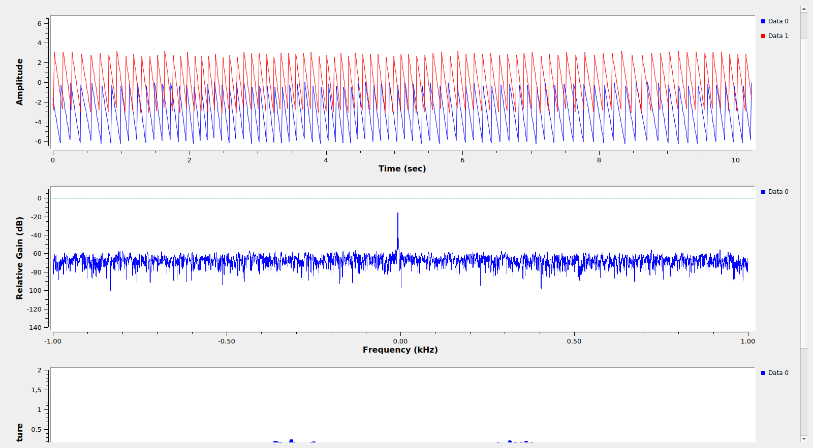
From the software side, I am using my limesdr_linrad tool from the qo100-groundstation repository and GNU Radio. This GNU Radio flowgraph generates the CW tone so that it ends up 5kHz below the BPSK beacon frequency and performs phase measurements of the tone and the BPSK beacon on the downlink. The phase of the tone is measured with a PLL, while the phase of the BPSK beacon is measured with a Costas loop. Phase measurements of each of the signals are written to a file at a rate of 100Hz. The file is then processed in this Jupyter notebook to compute and plot Allan deviation.
The measurement test was made on 2019-11-10, between 11:10 and 11:20 UTC. A continuous CW tone was transmitted approximately 5kHz below the BPSK beacon. Its power was adjusted so that the downlink power was 2dB lower than the BPSK beacon. The phase measurements obtained during the tests are in this file. It is somewhat longer than the 10 minutes that the test lasted “officially”, since I started a bit earlier in order to transmit a CW identification with my callsign and ended up a bit late to transmit another CW identification.
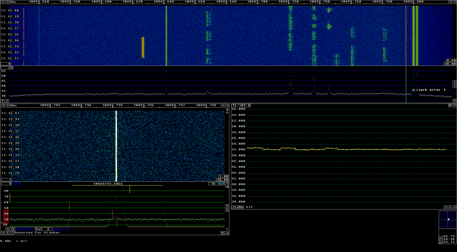
The figures below show the GNU Radio flowgraph performing the phase measurements during the test and Linrad monitoring the transponder downlink. Note that Linrad was only used for monitoring, and not involved in the measurement process.
The plot of the Allan deviation of the measurements is shown below. Note that to compute the Allan deviation of a time series of clock comparisons, you need to know the frequency at which these clock comparisons were made. The equations above show that the CW-BPSK measurements were done at a frequency of 2.4GHz, while the CW measurements were done at 8GHz. The BPSK measurements involve several clocks and frequencies, so it is not clear what to do without further considerations. However, if we use 10GHz as the measurement frequency for the BPSK measurements (as done in the plot below), we see that the three traces line up neatly for \(\tau > 0.5\mathrm{s}\).
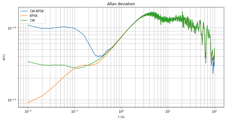
For the interpretation of these results, first we know that the CW-BPSK and CW measurements have roughly the same deviation. The clock which appears in both measurements is my station’s clock \(t_{\mathrm{EA}}\). This means that my station clock is less stable that the clocks at Bochum or QO-100, so it can’t possibly be used to measure the QO-100 LO. Since \(t_{\mathrm{EA}}\) is less stable than the two other clocks, it is the dominating term in \(\varphi_{\mathrm{BPSK}}\). This justifies our choice of 10GHz as the measurement frequency when computing the Allan deviation for the BPSK measurement, since \(\varphi_{\mathrm{BPSK}}\) turns out to be a measurement at 10GHz of my station’s clock.
In conclusion, my clock is less stable than the clocks at Bochum or QO-100, so the Allan deviation shown for \(\tau > 0.5\mathrm{s}\) is just a measurement of the Allan deviation of my clock. At least this measurements place an upper bound on the stability of the QO-100 local oscillator. We see that it is better (probably much better) than \(7\cdot10^{-11}\) for \(\tau = 1\mathrm{s}\).
There seems to be interesting data about phase noises in the Allan deviation for \(\tau < 0.1\mathrm{s}\), but I haven’t done an interpretation of that data.
It would be interesting if other stations with more stable clocks can participate in this kind of measurements. A good OCXO would be ideal for this kind of short-term stability measurements.
3 comments