This post is a follow up to my experiments about measuring the stability of the QO-100 NB transponder local oscillator. I am now using the Vectron MD-011 GPSDO that Carlos Cabezas EB4FBZ has lent me to reference all my QO-100 groundstation (see more information about the Vectron GPSDO in this post).
The Vectron MD-011 has an Allan deviation of \(10^{-11}\) at \(\tau = 1\,\mathrm{s}\) and \(2\cdot10^{-11}\) at \(\tau = 10\,\mathrm{s}\) according to the datasheet, so it is an improvement of an order of magnitude compared to my DF9NP TCXO-based GPSDO. I have made more measurements with the Vectron MD-011 as in my previous experiments, measuring the phase of the BPSK beacon transmitted from Bochum and a CW tone transmitted with my station. This post summarizes my results and conclusions.
Long measurement of the BPSK beacon
The first experiment I did was a long measurement of the BPSK beacon phase. Recall from the previous post that this measurement is harder to interpret, since it involves three clocks measured a different frequencies: my station clock, the clock at Bochum, and the transponder local oscillator. Additionally, for long measurements, the satellite movement with respect to the groundstations needs to be taken into account.
The measurement was done on October 21 and 22, spanning a bit over 41 hours. The test_bpsk_beacon.grc GNU Radio flowgraph was used to recover the carrier phase of the beacon with a Costas loop (with 10Hz bandwidth) and write phase measurements at a 100Hz rate. These measurements are analyzed in a Jupyter notebook.
The figure below shows the BPSK beacon frequency offset. The 0Hz level in the graph is set arbitrarily so that the trace is more or less centred at zero. The daily sinusoidal Doppler curve can be seen easily. The frequency averaging period in this graph is 1 second.
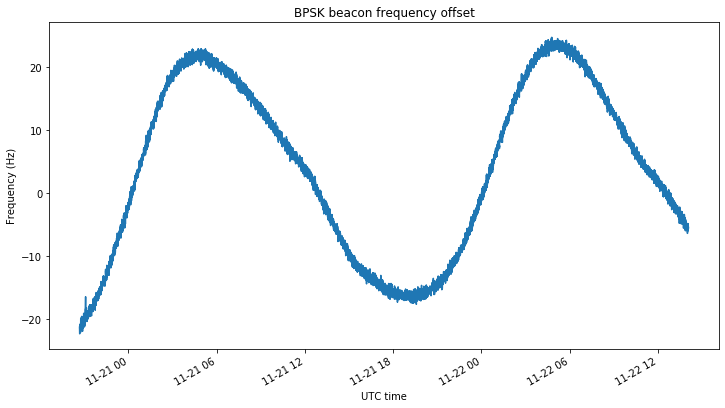
The Doppler of Es’hail 2 has been thoroughly studied in several posts in this blog. For instance, this post shows some frequency measurements of the BSPK beacon done back in March. The Doppler curve resembles a sinusoidal curve with a period of one (sidereal) day and an amplitude of approximately 2ppb (or 20Hz). Most of the Doppler on the BPSK beacon is due to the downlink Doppler, owing to the large frequency ratio of 4.37 to one between downlink and uplink frequencies.
The Allan deviation is computed using the method of overlapping segments. It is shown in the figure below.
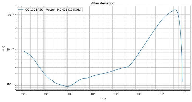
For \(\tau\) between 1 and 10 seconds the deviation is already limiting the measurement capabilities of the Vectron GPSDO. For \(\tau > 3\cdot 10^2\,\mathrm{s}\) we see the effects of Doppler starting to dominate, increasing the deviation a lot. When \(\tau\) equals one sidereal day, the Allan variance should drop a lot, because of the quasi-periodicity of the Doppler. This effect can be seen at the right-hand side of the figure.
Measurements of a CW tone and BPSK beacon
The next experiments involved the measurement of the phase of the BPSK beacon transmitted by Bochum and a CW tone transmitted by my station simultaneously, in the manner described in this post. Three observations lasting between 14 and 45 minutes were made in different moments of the day on October 22 and 23.
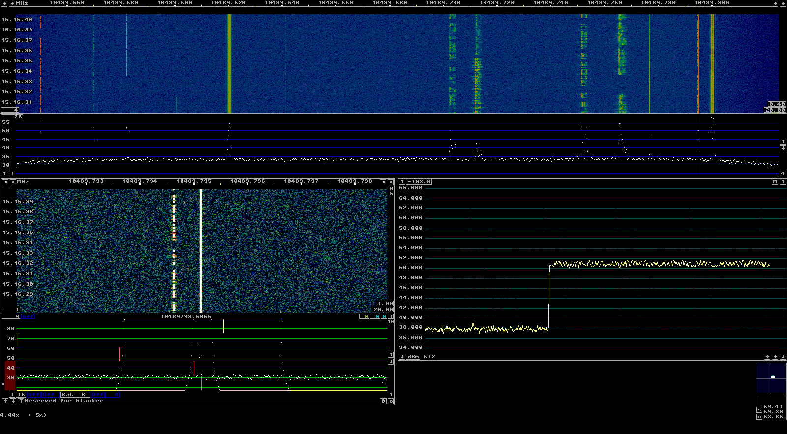
To comply with the requirement to identify the transmissions, my signal consisted of a continuous CW tone transmitted at 2400.295MHz for the phase measurement and a telegraphy signal looping the message EA4GPZ FREQ TEST transmitted 500Hz below the main CW tone. This telegraphy signal was 6dB weaker than the main tone. The downlink power of the main tone was some 3dB weaker than the BPSK signal.
The GNU Radio companion flowgraph test.grc is used to transmit the measurement signal and take phase measurements. The phase of the BPSK beacon is detected with a Costas loop, while the phase of the CW tone is tracked with a PLL. Both use a bandwidth of 10Hz and the measurement frequency is 100Hz. The results are processed in this Jupyter notebook.
The figure below shows the phase measurement signal during one of the tests.
As explained in the previous post, by subtracting the phases of the CW tone and BPSK beacon, a comparison of the clocks at my station and Bochum at an observation frequency of 2.4GHz is obtained. The figure below shows the clock difference in nanoseconds for each of the three observations.
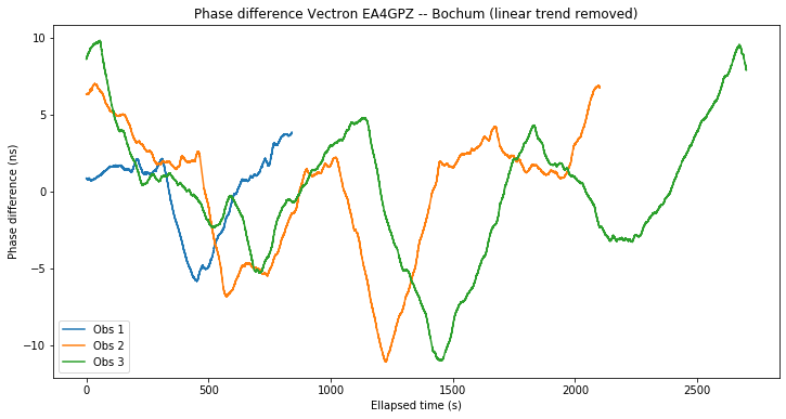
The difference reaches values of up to +/-10ns. This might seem large, since a good GPS receiver can compute a timing solution with a noise of perhaps 2 or 3ns. The reason for the variations much larger than 3ns is interesting. While the GPS solution can be rather precise, it is also very noisy, meaning that it varies significantly from epoch to epoch. If the GPSDO was to follow its timing solution closely, the short-term Allan variance would be horrible. Thus, the GPSDO pulls the OCXO slowly, to keep the short-term Allan variance as good as that of the free-running OCXO.
By letting the GPSDO phase difference grow up to 10ns, the Allan variance is kept smaller than by trying to make the difference as close to zero as possible. The Vectron GPSDO shows this quite well in a screen that shows the output offset with respect the timing solution and the OCXO DAC voltage. The offset often reaches 10ns, and the DAC voltage changes only after several seconds.
To analyse the Allan deviation we follow the same approach as in the previous post, except for the fact that the method of overlapping segments is used. The difference between the CW tone and the BPSK beacon is considered as a clock comparison between my station and Bochum at a frequency of 2.4GHz. The CW tone is considered as a clock comparison between my station and the QO-100 NB transponder local oscillator at a frequency of 8.1GHz. The BPSK frequency involves the three clocks at different frequencies, and is considered at a frequency of 10.5GHz (as the expression involves my station clock at this frequency).
The Allan deviation of the three observations is shown below. For reference, the deviation of the long observation of the BPSK beacon is shown in red.
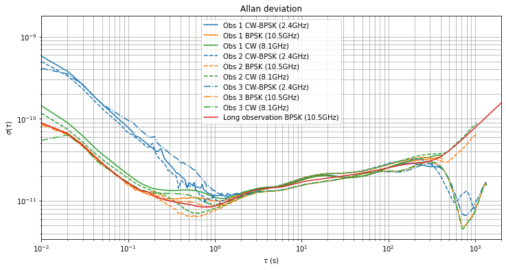
Between \(\tau = 1\,\mathrm{s}\) and \(tau = 2\cdot10^2\,\mathrm{s}\) we get roughly the same results in all the observations and for all the three measurements (CW-BPSK, BPSK and CW). According to the discussion in the previous post, this means that the clock at my station is again the least stable clock in the system. This has come to me as a surprise.
After obtaining these results, I have asked Achim Vollhardt DH2VA what kind of GPSDO is used to generate the BPSK beacon in the AMSAT-DL groundstation in Bochum. He tells me that it is an HP Z3801A. This information also appears in the description of the hardware at the Bochum 20m antenna.
Apparently the Z3801A is one of the best GPSDOs ever made, and its Allan deviation at \(\tau = 1\,\mathrm{s}\) can reach \(10^{-12}\). This page shows an Allan deviation plot of the Z3801A, both locked and unlocked, and this page compares the Allan deviation of several unlocked Z3801A units. In view of these results, it is quite likely that the Bochum clock has an Allan deviation around or below \(10^{-12}\), so it is an order of magnitude better than the Vectron GPSDO I’m using.
Often the short-term stability of an OCXO is quoted to be \(10^{-11}\), so in this respect the OCXO in the Vectron GPSDO is average. It seems that the Z3801 uses a really good OCXO that in many units achieves performance around \(10^{-12}\). It is hard to beat this stability for \(\tau = 1\,\mathrm{s}\). A Rubidium standard will be around \(10^{-10}\) for short-term, and a Cesium standard will often be at \(10^{-12}\). A Hydrogen maser is needed to get significantly below \(10^{-12}\).
The details about the clock used in the QO-100 transponder are under NDA. The results of my experiments show that it is probably well below \(10^{-11}\) for \(\tau\) between 1 and 100 seconds.
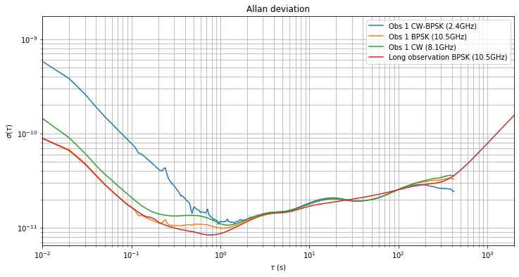
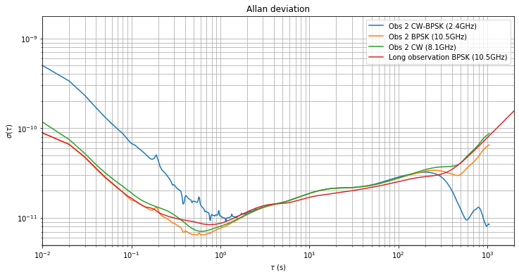
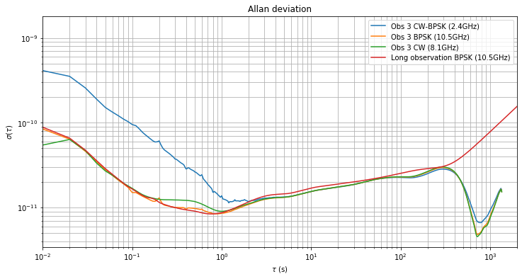
The Allan deviation of each of the observations is shown below in separate figures for an easier comparison. While the first observation is too short to examine the medium-term behaviour for \(\tau\) bewteen \(10^2\) and \(10^3\) seconds, the other two observations show significantly different behaviour. These differences are caused by different Doppler behaviour and will be examined in the next section.
Effects of Doppler on medium-term measurements
We have seen that for \(\tau > 2\cdot10^{2}\,\mathrm{s}\) the effects of Doppler start being noticeable. First let us discuss how each of the three different measurements are affected by Doppler. We denote by \(d_E\) and \(d_B\) the Doppler between Es’hail 2 and my station (EA4GPZ) and between Es’hail 2 and Bochum respectively, measured in parts per one.
For the CW-BPSK measurement, only the Doppler in the uplink legs is important, since the downlink leg is common for the CW and BPSK signals, so the downlink Doppler is cancelled. Also note that the two Dopplers act with opposite sign: a positive \(d_E\) makes the CW signal appear higher in frequency, while a positive \(d_B\) makes the BPSK signal appear higher in frequency. Thus, the total Doppler on the CW-BPSK measurement is \(f_U(d_E – d_B)\), where \(f_U\) is the uplink frequency. Since this measurement is considered at an observation frequency of \(f_U\), the Doppler is simply \(d_E – d_B\).
For the CW measurement, only the Doppler at EA4GPZ plays a role. Since the transponder is non-inverting, the Doppler on the uplink and downlink legs adds up, so the total Doppler is \((f_U + f_D) d_E\). Since this measurement is considered at an observation frequency of \(f_L\), the Doppler is \((f_U+f_D)d_E/f_L\). The factor \((f_U+f_D)/f_L\) is approximately 1.59.
For the BPSK measurement, the Doppler at Bochum plays a role at uplink, while the Doppler at EA4GPZ plays a role at downlink. Both Dopplers act with the same sign: a positive Doppler either at Bochum or EA4GPZ will make the BPSK beacon frequency appear higher. Therefore, the total Doppler is \(f_U d_B + f_D d_E\). Since this measurement is considered at an observation frequency of \(f_D\), the Doppler is \(f_U/f_D d_B + d_E\). The factor \(f_U/f_D\) is approximately 0.229.
The figure below shows the Doppler at EA4GPZ and Bochum in parts per billion. We see that the Doppler curves are very similar.
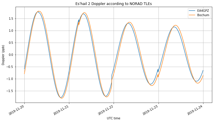
This similarity is caused by the motion of Es’hail 2 and the geometry between the stations and the satellite. The motion of Es’hail 2 is shown below in latitude, longitude and altitude coordinates. We see that its motion is a sinusoidal curve with an amplitude of 0.04 degrees in latitude and longitude, which corresponds to 27km at an orbital radius of 38000km, and 7km in altitude.
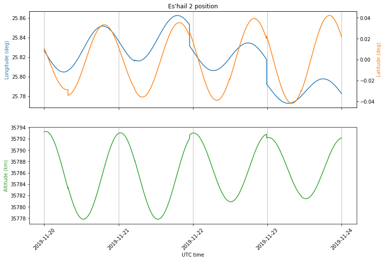
However, taking into account the geometry of the problem, we see that most of the Doppler comes from the variations in altitude, and so the Doppler is similar for all stations in the footprint. Since the Earth radius is small compared with the orbital radius, the line-of-sight vector for any groundstation is close to the vector between the Earth centre and the satellite. Indeed, all the groundstations lie within 9.7º off-nadir as seen from the satellite.
This means that the effect of horizontal (latitude and longitude) movement on the Doppler is reduced significantly. Moreover, Madrid and Bochum are relatively close, so the Doppler due to horizontal movement seen in both stations is similar. More information about the effect of Es’hail 2 movement in Doppler can be found in this post.
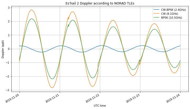
Taking into account the remarks above about how Doppler affects each of the three different measurements, we get the following figure. Since the CW-BPSK Doppler equals \(d_E – d_B\) and \(d_E\) and \(d_B\) are similar, it is much smaller than the others. Assuming that \(d_E = d_B\), we have that the CW Doppler is 1.29 times the BPSK Doppler.
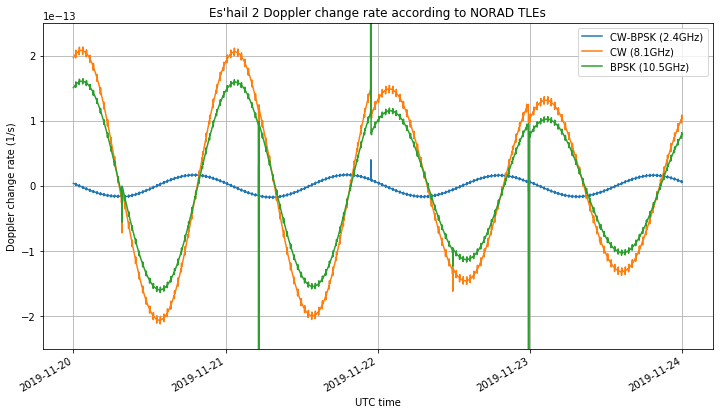
Allan deviation is not sensitive to frequency offset, but rather to frequency drift. Therefore, it is affected by Doppler change rate. In fact, for a frequency drift of \(a\) 1/s, the Allan deviation is \(a\tau/\sqrt{2}\). The figure below shows the Doppler change rate that affects each of the measurements. For the CW and BPSK measurement the change rate peaks at around \(10^{-13}\). Therefore, for \(\tau = 10^{2}\) the effects of Doppler start to be on the order of \(10^{-11}\) and are thus visible in the Allan deviation. The Doppler in the CW-BPSK measurement is much smaller.
The figures shown above have been obtained in this Jupyter notebook.
For medium-term measurements the Doppler change of rate can be assumed to be constant. Therefore, it can be estimated and removed by fitting a degree 2 polynomial to the phase measurements. As shown in the figure below, if we remove this quadratic term from the phase measurements, the Allan deviation of all the observations now decreases for \(\tau\) greater than \(2\cdot 10^2\,\mathrm{s}\), since most of the contribution of Doppler has been cancelled.
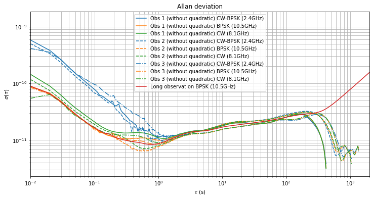
Observation 1 is perhaps too short for a good estimation of the frequency drift due to Doppler, but observations 2 and 3 give the following good estimates of the drift in units of 1/s:
- Observation 2: CW-BPSK \(8.96\cdot10^{-15}\), BPSK \(4.12\cdot10^{-14}\), CW \(5.60\cdot 10^{-14}\).
- Observation 3: CW-BPSK \(4.89\cdot10^{-15}\), BPSK \(-4.62\cdot 10^{-15}\), CW \(-4.52\cdot10^{-15}\).
We see that there is a difference of an order of magnitude in the drift of the BPSK and CW measurements between observations 2 and 3. The reason is that the observations were done at different moments of the Doppler curve. Observation 2 was made on 2019-11-22 22:08 UTC, when Doppler change rate was high. Observation 3 was made on 2019-11-23 17:10 UTC, when Doppler change of rate was low.
This explains the difference in the Allan deviations of observations 2 and 3. For observation 2, the Doppler in the BPSK and CW measurement is large and appears in the Allan deviation. However, the Doppler in the CW-BPSK measurement is too small to be noticeable, except for \(\tau > 6 \cdot 10^2\), when the deviation starts increasing again. In observation 3, the Doppler in all the three measurements is small, so the deviation decreases until \(\tau = 7\cdot 10^2\), when it starts to increase again.
Concluding remarks
These experiments have shown that the short-term stability of the QO-100 NB transponder local oscillator is better than \(10^{-11}\), so the Vectron MD-011 cannot be used to measure it. The GPSDO at Bochum seems much better than \(10^{-11}\), so perhaps measurements of the transponder local oscillator can be done by receiving the BPSK beacon at Bochum.
The short-term stability of the QO-100 NB transponder local oscillator is better than that of most Amateur stations. The idea to measure the stability of the transponder LO started with some questions from Amateurs interested in running VARA and other OFDM modes which need a lot of frequency stability through the transponder. These measurements show that the transponder is not the limiting factor when using modes that need frequency stability.
The effect of Doppler in the measurements has been studied. The frequency drift \(a\) is on the order of \(10^{-13}\) 1/s and contributes to the Allan deviation as \(a\tau/\sqrt{2}\), so for the measurement precision of \(10^{-11}\) that we are analysing here it starts playing a role for \(\tau > 100\,\mathrm{s}\). For a study down to \(10^{-12}\), the Doppler needs to be taken into account for \(\tau > 10\,\mathrm{s}\). However, for medium-term measurements the Doppler change rate can be assumed constant and cancelled by subtracting a quadratic term from the phase measurements.
Tks, CT1TO