32APSK narrowband modem for QO-100

Some time ago I did a few experiments about pushing 2kbaud 8PSK and differential 8PSK through the QO-100 NB transponder. I didn’t develop these experiments further into a complete modem, but in part they served as inspiration to Kurt Moraw DJ0ABR, who has now made a QO-100 Highspeed Multimedia Modem application that uses up to 2.4 kbaud 8PSK to send image, files and digital voice. Motivated by this, I have decided to pick up these experiments again and try to up the game by cramming as much bits per second as possible into a 2.7 kHz SSB channel.

Now I have a definition for the modem waveform, and an implementation in GNU Radio of the modulation, synchronization and demodulation that is working quite well both on simulation and in over-the-air tests on the QO-100 NB transponder. The next step would be to choose or design an appropriate FEC for error-free copy.

In this post I give an overview of the design choices for the modem, and present the GNU Radio implementation, which is available in gr-qo100_modem.

Modem design

Design criteria

The set of design criteria or requirements that I have taken for this modem are the following:

• The modem should fit into 2.7 kHz bandwidth, making it compatible with SSB voice from the point of view of spectrum management of the NB transponder.
• The modem should give error-free copy when its downlink power is adjusted to be the same as the BPSK beacon of the NB transponder, which is received at approximately 50 dB·Hz CN0 with a reasonable groundstation.
• The modem should work with a reasonably stable groundstation frequency reference, which can be an OCXO-based GPSDO, or perhaps even a TCXO-based GPSDO.
• The modem does not need to take multipath into account. The channel will be AWGN, plus the typical frequency drift given by the groundstation reference.

I think these are very reasonable requirements for this usage. Since the modem is a beacon-power 2.7 kHz signal, we comply with all the NB transponder bandplans. As we are trying to reach the limits of what is possible, we are assuming that the groundstation is well adjusted and uses current technology. In particular, the modem design will probably not work with:

• Stations that have a reference that drifts several tens of Hz.
• Conventional radios. Even though the modem fits in 2.7 kHz, a flat frequency response is assumed. Unless it is possible to accurately equalize the filters of a conventional radio, an SDR transceiver should be used.
• Badly adjusted stations that drive amplifiers into compression or have significant IMD. Good linearity is assumed.

One design criteria that I have decided not to treat is latency. I don’t want to compromise the design so much by targetting low latency, which forces short FEC codewords, and has other considerations regarding synchronization. I don’t want the modem to take several seconds to synchronize or decode a FEC codeword, either, but I think that the data rate is more important than latency. The round-trip-time for a GEO channel is already close to 0.3 seconds. I feel that trying to design a digital voice modem that supports short overs brings extra design considerations that will impact the data rate. So for this modem I’m mainly thinking about a continuous or long transmission to which the receiver can synchronize at any time.

Modulation and baudrate

For the design of the modem I’m taking a lot of inspiration from DVB-S2, since it is engineered very well to push data over an AWGN channel close to the Shannon limit. However, there are some aspects of the modem that need to be changed radically, since DVB-S2 is intended for much higher baudrates.

The modem is an APSK waveform with RRC filtering using an excess bandwidth of 5%. This is the smallest excess bandwidth supported by DVB-S2, and it is already a bit challenging to work with, since the RRC filter must be quite long and inter-symbol interference is significant unless the matched filter is implemented well. On the other hand, this low excess bandwidth allows us to use a higher baudrate while still fitting into 2.7 kHz. I have decided to use 2570 baud, which with an excess bandwidth of 5% has an occupied bandwidth of 2698.5 Hz, just under the target of 2.7kHz.

The next step is to choose the constellation. Table 13 in the DVB-S2 standard can be of help. It is reproduced here for convenience.

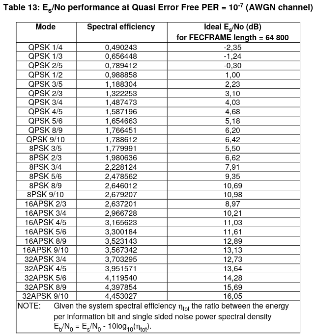
At a CN0 of 50 dB·Hz and a 2570 baud we have Es/N0 = 15.9 dB. Thus we see that we are around the target Es/N0 for the 8/9 and 9/10 32APSK DVB-S2 MODCODs. Thus, for our use case it seems reasonable to try to use 32APSK together with a good FEC that gives a rate around 8/9 or 9/10.

32APSK is the highest order modulation supported by DVB-S2, but DVB-S2X introduces even higher order modulations, as shown in the table below.

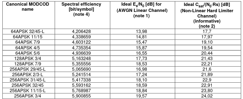
According to this table, it seems that 64APSK 4/5 might be a good option, but the spectral efficiency it gives is only slightly higher than 9/10 32APSK. Still, this is an area where there is some room for future improvement of the modem.

Pilot symbols

The most tricky part about the modem design is the frequency drift of the groundstation reference. The problem with having a rather low symbol rate is that reference symbols need to be inserted quite frequently. For instance, the scheme of pilot symbols used in DVB-S2 cannot be used, since pilot symbols would be spaced too far apart in time.

A related question is how much frequency drift we need to handle, since in the requirements above I have been quite vague. My post about the coherence time of a typical QO-100 groundstation can give a ballpark estimate. I think that we can safely assume that the drift will be tracked by a PLL with a bandwidth around 10 or 20 Hz. Moreover, since we are using a rather tight constellation, we need to have good loop SNR in the PLL. Perhaps we can aim for 20 dB of loop SNR. This means that it is sufficient to devote 30 dB·Hz of our total 50 dB·Hz budget to phase synchronization.

There are two ways to achieve this. The first is to have a 30 dB·Hz reference signal next to or on top of our waveform. This is a simple approach but it is somewhat unconventional (unless we think about residual carrier modulations). It is also not the best regarding bandwidth efficiency. Still, a 30 dB·Hz CW tone on one of the edges of the signal would not be a too bad idea.

The other way, which is the more common, is to transmit pilot symbols on 1/100 of the symbols. This has the problem that the pilots don’t appear very frequently. In the best case, we spread them apart, so that the first out of every 100 consecutive symbols is a pilot symbol, and so the pilot symbol rate is 25.7 baud. It isn’t too convenient to update the PLL loop, which has a bandwidth of 10-20 Hz, at a rate of only 25.7 Hz (recall that the product of loop bandwidth times update rate, typically called BT, should be a few times smaller than one).

Therefore, I have decided to make pilot symbols more frequent. In my design candidate, one out of 50 symbols is a pilot, so the pilot symbol rate is 51.4 baud, which already makes things much better for the PLL. I’m hesitant to increase the pilot symbol frequency much further, since this impacts the useful data rate, but this is a parameter that can still be fine tuned according to the results of over-the-air tests with stations having different frequency references.

For best performance, pilot symbols need to be modulated with a pseudorandom sequence, so that their contribution to the power spectral density is the same as that of the data symbols. I have decided to modulate pilot symbols using a BPSK 31-bit m-sequence.

It is perhaps more typical to use other modulations, such as QPSK, for the pilots. I think that the main reason is that a QPSK waveform has less zero crossings in average than BPSK, which improves the peak-to-average power ratio. For instance, in DVB-S2 the PLHEADER is modulated using \(\pi/2\)-BPSK. The pilot symbols are 36 consecutive \(\sqrt{2}/2(1 + i)\) symbols, but they are scrambled by multiplication with the PL scrambler, which is a QPSK sequence.

In our case, however, since the adjacent symbols of each pilot symbol are 32APSK data symbols, choosing a BPSK or QPSK constellation for the pilots would give the same amount of zero crossings in average. Moreover, since we are thinking about a continuous signal to which the receiver can synchronize at any time, a BPSK modulated m-sequence gives the optimal synchronization sequence by means of circular correlation.

The m-sequence has been chosen long enough to have a clear autocorrelation peak and good cross-correlation rejection with the random data symbols, but not longer than necessary. Having a longer m-sequence would mean that the m-sequence takes more time to transmit, which impacts the synchronization time if the receiver tries to acquire the signal by circular correlation with the complete m-sequence. I think that a 31-bit m-sequence gives a good balance, because it takes 603 ms to transmit, which is not too long compared with the GEO round trip time of some 270 ms.

Constellation

The DVB-S2 32APSK constellation is shown in the figure below. Its definition depends on two parameters \(\gamma_1\) and \(\gamma_2\) that give the relative radiuses of the three concentric PSK rings. It is interesting that the values of \(\gamma_1\) and \(\gamma_2\) depend on the coding rate, as indicated in the table below the constellation.

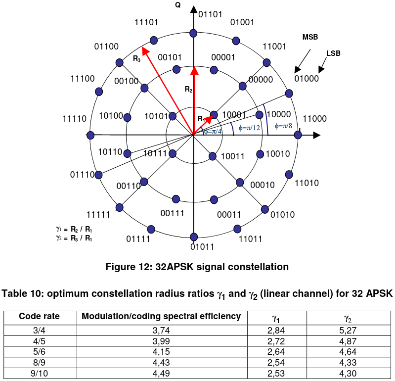
Lower coding rates use larger values of \(\gamma_1\) and \(\gamma_2\), which have the effect of making the outer rings larger and the inner ring smaller. For now I am using the values for coding rate 9/10 in my tests, but these parameters should be optimized when the FEC is chosen.

The 32APSK constellation needs to be normalized so that the average power, which is given by \((R_1^2 + 3R_2^2 + 4R_3^2)/8\) is one. The BPSK pilot symbols are chosen as +1 and -1.

There is actually additional freedom for trading power between the 32APSK data constellation and the BPSK pilot constellation. It is possible to multiply the the amplitude of the BPSK symbols by \(\alpha\) and the amplitude of the 32APSK symbols by \(\sqrt{(50-\alpha^2)/49}\) while maintaining the average power power of the waveform. Since there is more than enough power in the pilot symbols for the correct operation of the PLL, we could take \(\alpha < 1\), which reduces the power allocated to the pilot symbols and slightly increases the power allocated to the data symbols. The gains in data symbol power are small, since the power we rob from the pilots is spread over 49 data symbols. Therefore, I have decided to set \(\alpha = 1\), since robust synchronization is probably more important that having a little bit more power in the data symbols.

Waveform design summary

The following is a summary of the characteristics of the 32APSK waveform:

• Single-carrier APSK waveform
• Baudrate 2570 baud
• RRC filtering with excess bandwidth 5%
• Occupied bandwidth 2.7 kHz
• Pilot symbols in TDD every 50 symbols
• BPSK pilot symbols with 31-bit m-sequence
• 32APSK data symbols

Modulator implementation

I have decided to use 8 ksps IQ for the implementation of the modem in GNU Radio, since this is a typical sample rate that can be used to process a 2.7kHz SSB channel. The baudrate of 2570 baud is a bit of an oddball number (in fact 257 is a prime number), so I have decided not to implement the modem using a sample rate that is related to the baudrate by a simple fraction.

At 8 ksps, the samples per symbol is around 3.113. I have decided to use a Polyphase Arbitrary Resampler block to resample the symbols from 2570 baud to 8 ksps, while performing RRC filtering. As remarked above, with an excess bandwidth of only 5% it is critical that the RRC filters are implemented accurately, so I have decided to use 64 arms in the polyphase filter. The length of each of the arms is chosen according to the decay of the RRC taps. I have decided that 47 taps is a good choice.

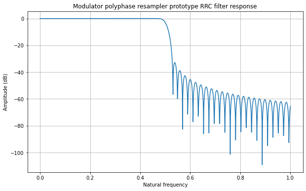
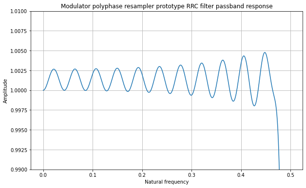
The figure below shows the prototype filter used for the modulator. As we can see, at 47 taps per filter arm the RRC response has already decayed significantly in the edges of the filter.

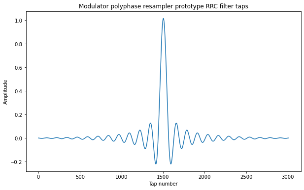
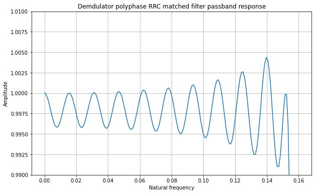
The frequency response of the prototype filter has around -35 dB of sidelobe attenuation. This is something that we could improve, but note that at 50 dB·Hz of CN0, the SNR in the occupied bandwidth is 15.7 dB, so the -35 dB sidelobes are already deep below the transponder noise floor.

The passband ripple of this filter is 0.5%.

The book by fred harris gives an interesting way to improve the response of a windowed RRC filter in Chapter 4.3, so that is a possible improvement for the future.

The modulator is implemented in a GNU Radio hierarchical flowgraph qo100_modulator.grc. The data comes in at 5 bits per byte, is mapped and modulated according to the 32APSK constellation, and multiplexed with the BPSK pilot symbols. Resampling and RRC filtering is done with the Polyphase Arbitrary resampler. Constants involved in the modem definition, such as the constellation, baudrate, etc., are defined in the Python module constants.py, since these are also used in the demodulator.

Demodulator implementation

Symbol synchronization

Since one of the challenges of making this kind of modem work correctly is the frequency drift, I wanted to decouple completely the symbol synchronization from the carrier recovery. Thus, I decided to perform first symbol synchronization and RRC matched filtering with the Symbol Sync block and then work with the pilot symbols already at one sample per symbol for carrier recovery.

The Symbol Sync block is configured with a polyphase filterbank implementing a matched filter and the maximum-likelyhood TED. This works OK, and in fact is able to synchronize quickly in my over-the-air tests. However, the performance is not so great. The clock recovery is too sensitive about the loop bandwidth, and sometimes the clock phase seems to slip slightly, causing some inter-symbol interference. Therefore, this is one of the aspects of the receiver to improve in the future, perhaps by using the know pilot symbols to aid the clock recovery.

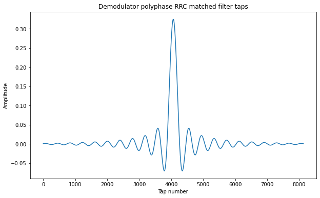
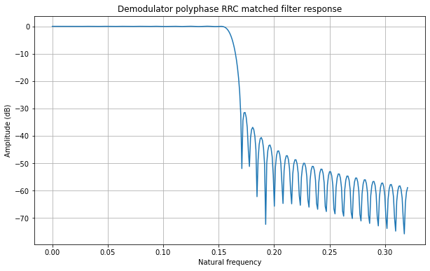
I have followed the same approach to design the prototype RRC filter of the Symbol Sync block as in the modulator. I am also using 64 arms in the polyphase filter and this time I am using 127 taps per arm, because the RRC time-domain response is roughly 3 times wider. The impulse response and frequency response of the filter are included in the figures below, which show similar performance to the modulator filter.

Carrier recovery

Carrier recovery uses the BPSK pilot symbols only. It is divided into two steps:

• An acquisition step that correlates against the 31-bit m-sequence to find the start of the pilot symbol sequence and produce phase and frequency estimates to bootstrap the PLL.
• A PLL that uses only pilot symbols to compute the phase error and wipes-off the known m-sequence that modulates the pilots.

These run on the stream of symbols produced by the Symbol Sync block.

The acquisition performs the circular correlation of a window of 31*50 symbols against the known 31-bit m-sequence used to modulate the pilot symbols in order to find the start of the pilot symbol sequence. The correlation is implemented using FFTs. In order to search in frequency, a circular shift in the frequency domain is done. All frequency bins are searched simultaneously. To have more frequency resolution, zero padding is done, duplicating the size of the FFTs to perform.

From the correlation peak we obtain the starting position of the pilot symbol sequence, and phase and frequency estimates. These are sent to the PLL using stream tags in the GNU Radio implementation. The PLL uses this data to keep track of the positions of the pilot symbols and to initialize the closed loop.

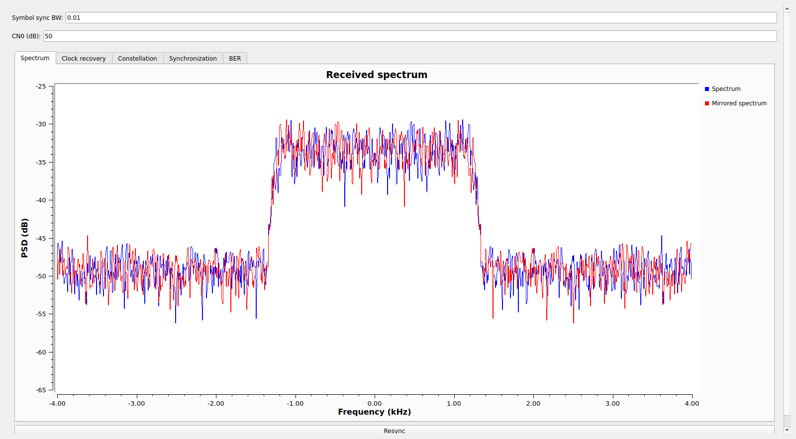
Note by the design of the waveform any algorithm that performs the correlation of the 31-bit pilot symbol m-sequence will only be able to detect frequency offsets in the ±25.7 Hz range, since the pilot symbol rate is 51.4 Hz. Larger frequency offsets will alias. Therefore, for the correct operation of the receiver it is necessary that the user tunes the signal to within ±25 Hz. As long as the groundstation frequency reference is stable enough, this is easy to do manually just by looking at the spectrum of the signal, which indeed has steep skirts due to the small excess bandwidth of the RRC filter. To help the user, the GNU Radio demodulator GUI plots both the spectrum of the signal and its mirror image. Only when the skirts of these two match well, the signal is correctly tuned. An improved decoder would perform this tuning automatically.

Note that this ±25 Hz frequency error limit refers only to the initial signal acquisition. When the PLL is tracking the carrier, the frequency error may drift further.

Since the acquisition block needs a window of 31*50 samples (in fact 31*50*2 samples in the current implementation, due to the FFT zero padding), it introduces a latency of 0.6 seconds (or 1.2 seconds) in the processing. In the GNU Radio implementation, in order to get lower latency this only happens until the correlation peak is found. After that, the acquisition block just lets samples through as they come in, introducing no latency. The block has a message port that can be used to resynchronize when necessary. Currently this resynchronization is triggered manually by the user with a GUI button, but in the complete modem it could be triggered by the FEC, or by the PLL.

The PLL includes a first order (phase and phase-rate) closed loop that uses the pilot symbols to track the carrier phase of the signal. It keeps track of what is the current received symbol, and when it receives a pilot symbol it wipes-off the m-sequence modulation and uses the phase error to update the loop filter. In its GNU Radio implementation it outputs the phase corrected data and pilot symbols on separate output ports, since after carrier recovery we would typically only care about data symbols.

At this stage, I have adjusted the coefficients of the loop filter by hand to get something that works more or less well with over-the-air tests. In the future I intend to use the ideas in the paper “Controlled-root formulation for digital phase-locked loops” by S.A. Stephens and J.B. Thomas. In this paper they analyse the design of the loop filter directly in discrete time, rather than porting a continuous time design to discrete time by using the bilinear transform. This is advantageous specially for large loop BT, which is the case for this receiver.

The PLL also includes an AGC that uses the pilot symbols as an amplitude reference. Even though there is an AGC earlier in the chain, as the Symbol Sync block requires normalized amplitude, this AGC is able to scale the amplitude more accurately.

GNU Radio implementation

Since the performance of the acquisition and PLL were an important part of the modem waveform design, they were prototyped in Python in this Jupyter notebook and tested with over-the-air recordings before being implemented as GNU Radio C++ blocks.

The figure below shows the GNU Radio implementation of the demodulator as a hierarchical block. The first block is a low pass filter that lets only 3 kHz of bandwidth. Then there is the RMS AGC block from gr-satellites that adjust the amplitude so that the signal has power one. Next we have the Symbol Sync block as described above.

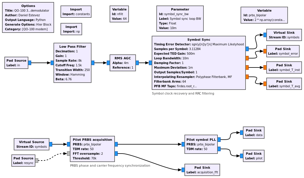
Then we have the Pilot PRBS acquisition block, which is a custom C++ block from the gr-qo100_modem out-of-tree module. This implements the FFT-based acquisition algorithm of the pilot m-sequence described above. Its first output is the stream of symbols, with tags corresponding to the synchronization peaks found. Its second output gives the FFT for the frequency bin where the maximum peak is found. This can be displayed in a GUI.

Finally we have the Pilot symbol PLL block, which implements phase tracking of the pilot BPSK symbols. Its first output gives the phase corrected data symbols, and its second output gives the phase corrected pilot symbols.

BER measurement

For measuring bit error rate, a fixed pseudorandom pattern is transmitted. This pattern is given in a data file. In order to keep synchronization to the pattern simple, the length of the pattern is 31*49 symbols, so that the pattern repeats every time that the pilot symbol m-sequence starts again. Since the PLL block knows the alignment with the m-sequence, it also knows the alignment with the pattern, and marks the first data symbol following the first pilot symbol with a stream tag.

These stream tags are then used to align the received data to the data file, using the Tags to PDU block from gr-pdu_utils. This is probably not the most efficient way to do it, but it is simple to implement.

The BER measurement is done in the GNU Radio hierarchical block shown below. Symbols are decoded using the nearest neighbour from the constellation. After correct alignment with the stream tags, the received data is compared with the reference data and bit errors are counted in windows of 10000 received bits.

Demodulator GUI

The demodulator is embedded in a QT GUI hierarchical flowgraph that plots all its inner workings, so that the user can evaluate the performance. This is shown in the figure below.

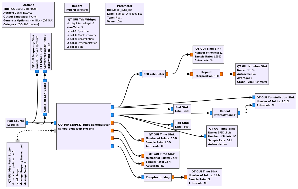
The GUI uses tabs to separate the different parts of the demodulator, since there are many plots. The following figures show each of the tabs running on a simulated signal with 50 dB·Hz CN0.

The first tab shows the spectrum of the signal. The mirrored spectrum is also shown to help the user tune correctly. When the sharp skirts of the signal and its mirror overlap, the signal is well centred.

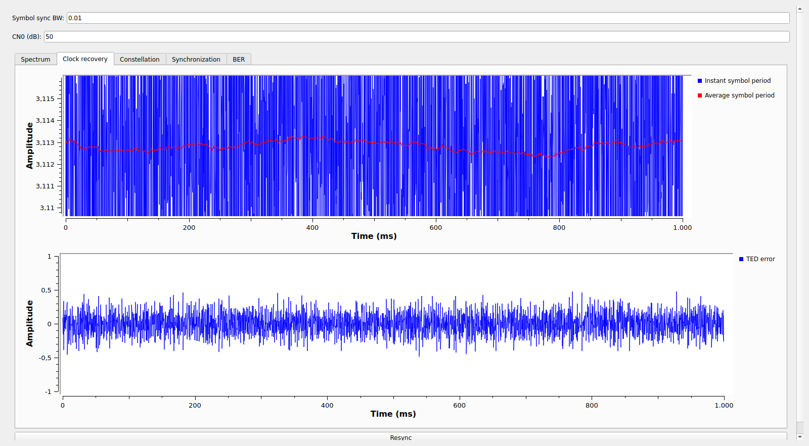
The next tab shows the clock recovery data. These are just plots of the output of the Symbol Sync block, which gives the average and instant symbol period and the TED error signal.

The constellation tab shows the 32APSK data constellation in blue and the BPSK pilot constellation in red. At 50 dB·Hz of CN0 the 32APSK constellation points start to merge, so it is easier to look to the BPSK constellation points to examine the quality of the signal.

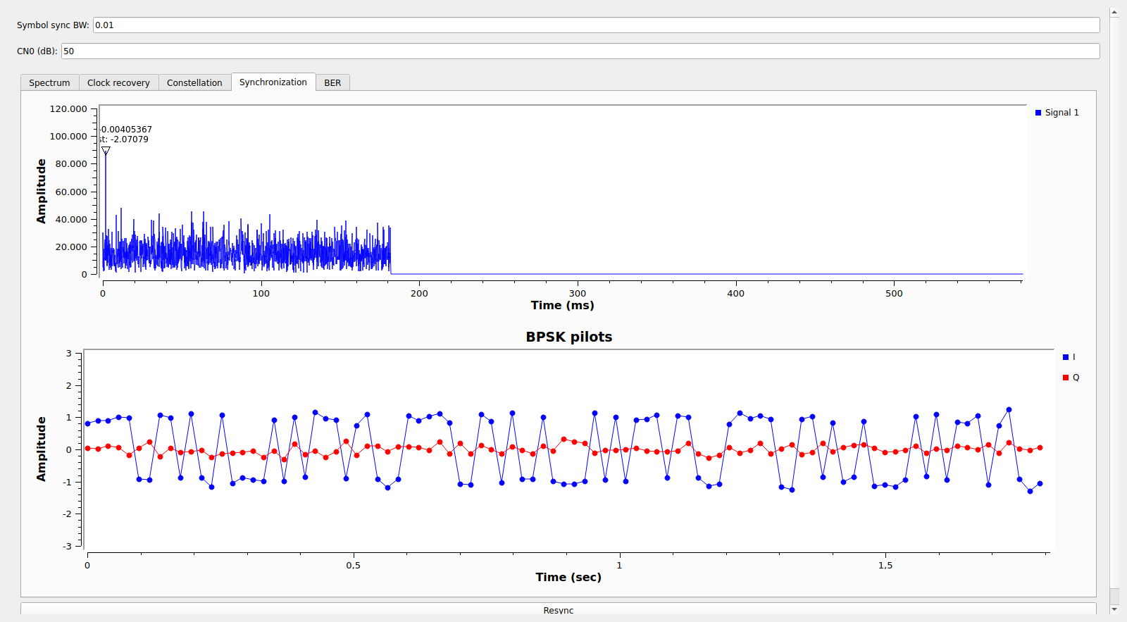
The synchronization tab shows the output of the FFT used in the synchronization algorithm on the top and the BPSK pilot symbols versus time on the bottom. The top plot only has data when the correlation is running (which is only until a peak has been found). Here we can see a large correlation peak.

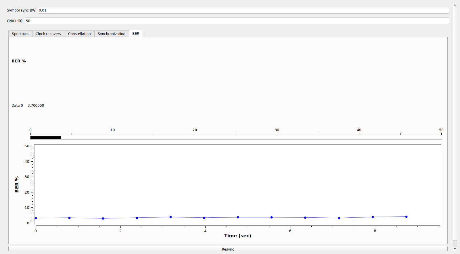
Finally, the BER tab gives the BER as a number that updates relatively fast (every 0.8 seconds) and as plot giving the history of the last 8 seconds.

The GUI has a Resync button at the bottom which the user can press if synchronization is lost. This will enable again the FFT-based synchronization.

Modem tests

My first tests to validate that the design of the modem waveform was reasonable were done with simulated signals with the target CN0 of 50 dB·Hz. I implemented the modulator in GNU Radio as described above, used an AWGN with frequency offset channel model (the Channel Model block) and the Symbol Sync to demodulate the data. The carrier synchronization algorithms were prototyped and tested in this Jupyter notebook.

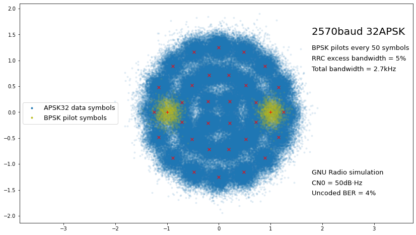
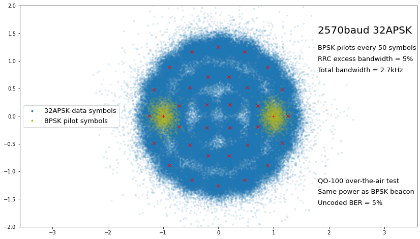
The results of the simulation were quite good. The constellation plot shown below summarizes the waveform design and the test results. I used this to show my design and the progress of my tests in Twitter. The BER is around 4%.

Next I passed to over-the-air tests on the QO-100 NB transponder, still using the prototype in Python. I run the GNU Radio transmitter in real time, and I made IQ recordings of the downlink signal for post processing. As usual, the groundstation hardware consisted of a LimeSDR mini for the uplink and the downlink IF, and a Ku-band LNB, with eveverything locked to a GPSDO reference.

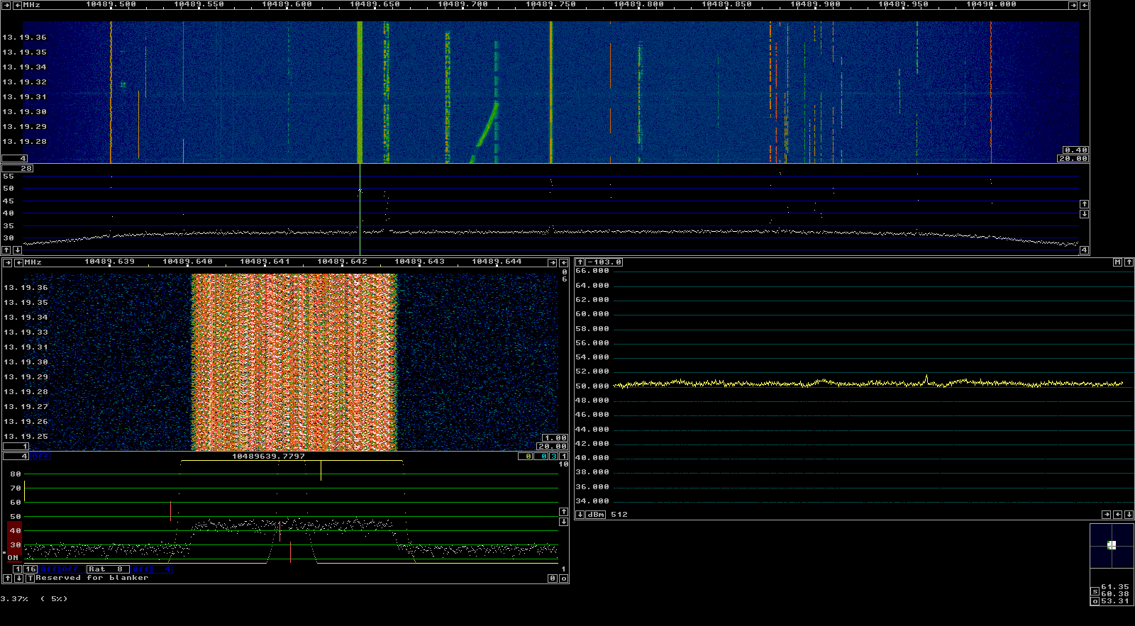
The figure below shows Linrad monitoring the test signal. The power has been adjusted so that the downlink power is slightly below the power of the BPSK beacon. The spectrum of the signal shows a noticeable pattern because with the test data for BER testing the signal repeats every 0.6 seconds. When random data is sent, the spectrum looks completely smooth.

The figure below shows the results of the over-the-air test processed with the Python prototype of the algorithms. The results are very similar to the simulated test. The constellation might seem slightly more noisy, but that is just because there are more symbols plotted. The IQ recording of this test can be found here.

The results of the first over-the-air tests were quite encouraging and convinced me that this was a reasonable design for the modem waveform.

It is worth to mention that the frequency reference that I’m using with my groundstation in the over-the-air tests is quite stable. It is the Vectron-MD011 OCXO-based GPSDO that I have used in these experiments (and several others). Moreover, since I’m using the same clock for the uplink and downlink, I’m seeing only 77% of the drift that I would see if I was receiving another station (the uplink drift cancels out part of the downlink drift). It will be interesting to see how the modem performs with less stable frequency references, but for this it makes sense to improve the PLL loop filter as described above.

After being happy with the performance of the waveform and the carrier recovery algorithms in Python, I ported these algorithms to GNU Radio C++ blocks, creating the gr-qo100_modem out-of-tree module to hold them. Then I re-organized my rather messy test flowgraphs into the hierarchical flowgraphs that I have described above.

In its present state, gr-qo100_modem gives example flowgraphs that can be used to run the modulator and demodulator and measure BER in the following scenarios:

• A simulated AWGN channel model
• Playback of the provided IQ recording
• Over-the-air test with SDR hardware

The over-the-air test that is included is prepared to work with my QO-100 groundstation software stack. The SDR sample rate is 600 ksps and the samples are sent to the radio by TCP and received by UDP using the Linrad protocol. This flowgraph needs to be adapted to work with other SDR hardware.

At this stage of the project, tests are greatly encouraged. If anyone is interested in setting up the GNU Radio software, or wants me to put a test signal in the QO-100 NB transponder, just let me know.

Next steps: adding FEC

The next step is to find or develop a suitable FEC that gives error-free copy with the typical 5% BER that I’m finding in my tests. As I have mentioned above regarding the BER tests, the 31-bit m-sequence gives a framing structure of 1519 data symbols (7595 bits). It would be nice if the FEC codewords were 7595 bits long, so that no additional synchronization markers would be needed to find the beginning of the codewords.

DVB-S2 normal FECFRAMES are 64800 bits long, and short FECFRAMES are 16200 bits long. Longer FEC codewords give better performance, but I think that 7595 bits will already give some decent performance. For instance, the CCSDS AR4JA LDPC code with 4096 information bits is said to perform only 0.6 dB worse than the equivalent code with infinite block size (see the discussion in Section 8.1 of the TM Synchronization and Channel Coding Green Book). Moreover, 7595 bit codewords already take some 0.6 seconds to transmit, so I wouldn’t like to make the codewords much longer than this.

The target coding rate I aim for is around 8/9 or 9/10. This idea is supported by the MODCOD tables of DVB-S2 included above. Taking into account the pilot symbols, such coding rates would give an information rate of 11194 or 11334 bps, which is not at all bad for a 2.7 kHz SSB channel. Thus, I think it’s reasonable to expect a user data rate of 11 kbps for this modem.