Last weekend, AMSAT-DL started some test transmissions of a high-speed multimedia beacon through the QO-100 NB transponder. The beacon uses the high-speed modem by Kurt Moraw DJ0ABR. It is called “high-speed” because the idea is to fit several kbps of data within the typical 2.7 kHz bandwidth of an SSB channel. The modem waveform is 2.4 kbaud 8APSK with Reed-Solomon (255, 223) frames. The net data rate (taking into account FEC and syncword overhead) is about 6.2 kbps.
I had never worked with this modem before, even though it served me as motivation for my 32APSK modem (still a work in progress). With a 24/7 continuous transmission on QO-100, now it was the perfect time to play with the modem, so I quickly put something together in GNU Radio. In this post I explain how my prototype decoder works and what remains to be improved.
Modem waveform
Kurt’s modem uses liquidsdr for all its DSP. It can use several constellations and baudrates. The configuration chosen for the beacon is 2.4 kbaud 8APSK. A root-raised cosine filter with an excess bandwidth of 0.2 is used as pulse shape filter.
The 8APSK constellation is a rather peculiar idea from liquidsdr (see here for all the constellations it supports). It consists of a point at zero and seven points equally spaced along a circle whose radius is chosen to give average power one (assuming that all the 8 symbols are equiprobable).
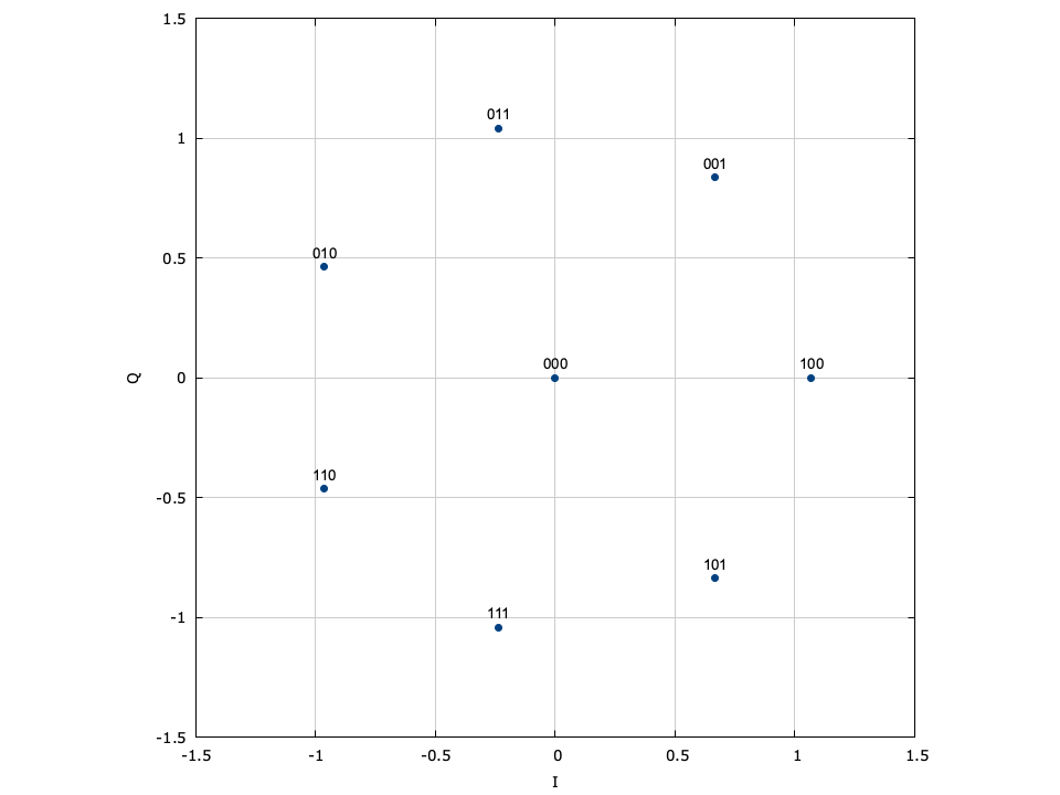
There were some comments in Twitter regarding what advantages and disadvantages this unusual 8APSK constellation gives over the usual 8PSK. I haven’t thought about this in much detail, and perhaps it’s worthy of a small study. The first clear difference is that in 8PSK all the constellation points have the same amplitude. This is not the same as the waveform having constant amplitude once we include an RRC pulse shape, but still helps reduce the peak-to-average power ratio. Probably 8APSK has somewhat higher peak-to-average power ratio due to its constellation point at zero.
Another difference is the distances between the constellation points. Here 8APSK wins, having larger distances. The consequence is that 8APSK has better BER performance at a fixed Eb/N0. In fact, the documentation of liquidsdr gives the following comparison of the 8-point constellations, where 8APSK is the best choice.

Another difference is carrier phase recovery. A Costas loop for 8APSK has less squaring losses than for 8PSK, since it essentially looks at the 7th (rather than the 8th) power of the signal to recover the suppressed carrier. On the other hand, for 8APSK only 7 out of 8 constellation points actually have information about the carrier phase. The point at zero can’t be used in the Costas loop. I don’t know which of these two effects wins (in the sense of which of the two constellations gives lower thermal noise in the Costas loop).
In the presence of phase noise (as it can be the case with the typical groundstations for QO-100), 8APSK should behave better, since the 7 points on the circle have larger phase differences than the 8 points from 8PSK.
A related topic is the efficiency of the Costas loop discriminant (phase detector). For 8PSK it is possible to implement a rather efficient discriminant, for instance as is done in GNU Radio. The technique is based on subdividing the 8PSK constellation in two 4-point constellations. It doesn’t seem possible to do something similar for 8APSK, in particular because 7 is a prime number.
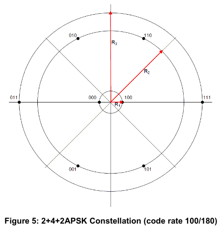
The choice of having an 8APSK constellation organized as 1+7 points is quite unique. I haven’t seen it anywhere else. For instance, DVB-S2X defines a 2+4+2 8APSK constellation where the 4 points in the middle ring are not equally spaced.
I have also seen 4+4 constellations and 2+6 constellations.
GNU Radio demodulator
The GNU Radio demodulator for this 8APSK constellation is shown below. The input runs at 6 ksps (I am including some downconversion and filtering before the demodulator, since I run my groundstation at 600 ksps). First, an AGC is used to normalize the signal to power one. Then the Symbol Sync filter performs clock recovery and RRC matched filtering using a polyphase filter. The maximum likelihood TED is used. It is important to use y[n]y'[n] instead of sign(y[n]y'[n]) even in high SNR conditions to prevent problems with the constellation point at zero.
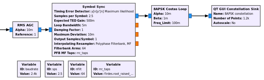
After the Symbol Sync there is an ad-hoc Costas loop for the 8APSK constellation implemented as a Python block. The work function of this block is really simple. It computes the angle of the output samples and multiplies it by 7 to obtain the error (this actually gives 7 times the carrier phase error in radians). There is a decision based on the amplitude used to ignore the constellation point at zero. The error is run through a second order loop filter. I’m eyeballing the values of the loop coefficients, and haven’t even bothered to set a particular damping factor.
def work(self, input_items, output_items):
  for j, x in enumerate(input_items[0]):
    output_items[0][j] = z = x * np.exp(-1j * self.phase)
    if np.abs(z) <= 0.5:
      error = 0
    else:
      error = (np.angle(z) * 7 + np.pi) % (2*np.pi) - np.pi
    self.freq += self.beta * error
    self.freq = np.clip(self.freq, -self.freq_limit, self.freq_limit)
    self.phase += self.alpha * error + self.freq
    self.phase = (self.phase + np.pi) % (2*np.pi) - np.pi
  return len(output_items[0])
This Costas loop works well, though it is not very efficient (but still runs in real time on my machine). The next thing I’ll do is to replace it by a C++ block that uses the control_loop class, as the usual Costas loop block does.
Synchronization and coding
For synchronization, a 24-bit (8-symbol) syncword is used. This is rather short and in fact the cross-correlation with other parts of the frame is relatively high. I think that a longer syncword (at least 16 symbols, ideally 32) would be a better choice.
The frames are Reed-Solomon (255, 223) codewords. Conveniently, 255 is divisible by 3, so each frame takes up an integer amount of symbols. The implementation by Kurt uses the Schifra Reed-Solomon library. The code and its parameters are taken directly from the example in Schifra’s documentation.
The Reed-Solomon codewords are scrambled with a synchronous scrambler. The scrambler sequence is defined by an array in scrambler.cpp. I haven’t tried to see if this sequence is the output of a suitable LFSR, but I think that this is likely.
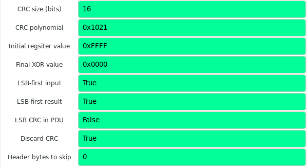
Each frame contains a CRC-16 at the end. The CRC code used is referred to as CRC16_MCRF4XX in this online calculator. It uses the CCITT polynomial.
Synchronization and FEC decoding in GNU Radio
Since the syncword is relatively short, reliable detection of the carrier phase ambiguity of the Costas loop using the syncword is difficult. Therefore, I have decided to do 7 decoder branches in parallel, one for each of the possible phase errors of the Costas loop.
The figure below shows one of the 7 branches in charge of the synchronization and FEC decoding. The blocks after the Sync and create packed PDU are shared by all the branches, since with PDUs we can do a many-to-one connection, but the other blocks are replicated 7 times.
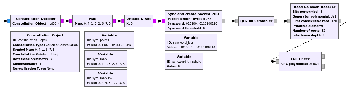
I have needed to use a Map block at the output of the Constellation Decoder because the decoder wasn’t using properly the symbol mapping from the constellation object. I haven’t looked at this problem in detail.
The way in which the syncword is found is not very good. The stream of 3 bits per symbol is unpacked and the syncword is then searched in the stream of bits. By doing this, we lose the information about the boundaries of the symbols. However, I don’t have a block that finds a syncword in a stream of non-binary symbols, so this was a convenient and quick way to do it.
The QO-100 Scrambler block is an ad-hoc Python block that contains the scrambling sequence. I will probably turn this into a C++ block. Or instead try to find the LFSR parameters that generate the sequence, to be able to use the Additive Scrambler.
The parameters of the Reed-Solomon code are taken directly from the Schifra example. The polynomial is the same as the one used in the CCSDS code, but the primitive element and first consecutive root are not.
Strangely, the first consecutive root is 120, which is the same as in the CCSDS (255, 239) code. The point of choosing such a first consecutive root instead of 1 for simplicity is to make the roots of the code generator polynomial \(g(x)\) invariant under the inversion \(z \mapsto z^{-1}\). This property makes the coefficients of \(g(x)\) symmetric, which reduces the number of calculations in the encoder.
In order to get this property, the first consecutive root should be \(128 – E\), where \(E\) is the number of errors that the code can correct. For \(E = 8\) (corresponding to a (255, 239) code) we get 120. However, for \(E = 16\) (corresponding to a (255, 223) code) we get 112. I don’t know why the Schifra example is using 120 with an \(E=16\) code, as this choice doesn’t seem to give any advantages.
Finally, the CRC is checked using the CRC Check block and the following parameters.
Higher protocol layers
The modem is mainly intended to send files. Therefore, the frame header is designed around this application. It is described in this page of the modem documentation. The frames contain a 2 byte header followed by 219 bytes of payload, which together with a 2 byte CRC give the 223 bytes of data for the Reed-Solomon encoder.
The header contains a 10-bit frame counter that counts the number of the block within the file that the frame carries. The 8 LSBs of this counter are in the first byte of the header, and the 2 MSBs are in the 2 MSBs of the second byte of the header.
Adjacent to the frame counter in the second byte there is a 2-bit frame status field. This is somewhat redundant and very similar to the CCSDS sequence flags (see for instance Section 4.1.3.4.2 in the Space Packet Protocol Blue Book). The status field indicates whether the frame is the first of a file split in multiple frames (which we can also see because the frame counter would be zero), a subsequent frame of a file, the last frame of a file (which we can also know given the size of the file, which appears in the first frame, and the frame counter), or the single frame for a small file (which we can also see looking at the frame counter and file size).
Finally, the 4 LSBs of the second byte of the header contain the frame type field. Different values indicate different types of files or data (image, HTML, etc.).
The way that files are transferred in the 219-byte payloads of these frames is explained here. Basically, the first frame of a file contains some metadata, including the filename and length, and the first 164 bytes of the file. The remaining frames contain 219 bytes of the file. In the last frame, the end is padded with zeros to reach 219 bytes if necessary.
Text, HTML and binary files are always sent as a compressed ZIP, so the ZIP needs to be extracted after being received.
To receive the files from the multimedia beacon, I have added a new class to the gr-satellites File Receiver. With very little code, this implements the protocol described above. All the logic is in the File Receiver itself, since I design it as a very general receiver that would support most ways of sending files by chunks.
Currently, there are two kinds of files being transmitted with the multimedia beacon. The first kind is ASCII text bulletins which are called amsat_1.blt, amsat_2.blt, etc. These contain news extracted from the AMSAT-DL website. The second type of file is the HTML page qo100info.html. This is the user interface for the streaming content of the multimedia beacon.
Websockets streaming data
Live data stream transmission is described in this page in the documentation. It works with an HTML file that is transmitted as described above and is used as the GUI for the streaming data. The modem runs a websockets server to which the browser viewing the HTML page connects to. All the packets with streaming data that are received by the modem (which are identified by the frame type 8) are sent through the websockets server. The HTML page includes some JavaScript to update the page and display the streaming information.
In the case of the QO-100 beacon, this feature is used to transmit spectrum and waterfall data, DX cluster spots, and the data from a CW skimmer. This streaming data represents most of the data bandwidth of the beacon.
I haven’t seen detailed documentation about how the websockets system works. The relevant part of Kurt’s code that handles it is this function. The type of data is identified by the first byte of the payload. We can see that DX cluster and CW skimmer payloads are sent directly to the websockets server, while spectrum and waterfall data are processed further by the modem before sending them.
So far I haven’t implemented anything about this streaming data feature, but I will probably do it, because it is the most useful and interesting part of the beacon.
Running the decoder
The GNU Radio flowgraph I’m using can be obtained here. This is still a prototype. In the future maybe I’ll add it to the examples folder of gr-satellites. The flowgraph requires the gr-satellites QO-100 multimedia beacon file receiver class, which at this moment is not included in any of the stable releases of gr-satellites, so you’ll need to build gr-satellites from the main branch.
This flowgraph is specific to how my station works. The input is a 600 ksps IQ stream using the Linrad network protocol. The beacon is downconverted and decimated to 6 ksps. Probably you’ll need to modify the first blocks in the chain to adapt them to your station.
The figure below shows the GUI of the GNU Radio decoder. In the spectrum plot I’m showing both the signal and its mirror image as a tuning aid: when the signal is centred, it coincides with its mirror image. The tuning frequency text box can be used to change the tuning and achieve this.
The syncword correlation plot shows how difficult it is to detect the syncword due to the high cross-correlation with the frame symbols. It shows the symbols corresponding to two full frames, so the location where the two visible syncwords are found doesn’t move with time (unless there are cycle slips). Watching this plot change for a few seconds makes it easier to see where the syncwords are, because the shape of their correlation doesn’t change, while the remaining parts of the correlation change due to the changes in the contents of the frames.
The decoder will store received files somewhere in the filesystem (by default it uses /tmp/). Additionally, it logs information about the number of errors corrected by the Reed-Solomon decoder and the whether the CRC checks are correct. With my station, the S/N of the signal is around 20 dB, so there are no bit errors and all the frames can be successfully decoded.
Estimado colega: te sigo desde hace tiempo. Enhorabuena por tus trabajos, desarrollos y difusión de los mismos. Sigue en ese camino. 73,s de Jabi, ea2aru.
very nice description, Daniel, thanks de DJ0ABR
Hi Daniel,
regarding the sync work. The relatively short sync word is just used to get an estimation when a frame could start. If it is really a frame or a false detect is checked by the decoder (CRC).
Would be nice to talk about various topics, maybe you want to write me an e-mail.
73 de Kurt DJ0ABR