In this post I continue with the analysis of an LTE downlink recording, which I started by looking at the primary and secondary synchronization signals. This recording is a one second excerpt of a 10 MHz cell in the B20 band that I recorded close to the base station, with a line-of-sight channel.
Now we will handle the reference signals to perform channel estimation. This will be used to equalize the received data transmissions. We will also handle the transmit diversity used by the base station, and show how to locate and demodulate some of the physical channels. All the calculations and plots are done in a Jupyter notebook.
The cell-specific reference signals (CRS) are transmitted in every subframe across all the cell bandwidth. They can be transmitted on either one, two or four antenna ports. In LTE, the concept of an antenna port does not necessarily correspond to a physical antenna. Signals are said to use the same antenna port if they have the same propagation channel to the user. Therefore, different beamforming combinations of the same physical antennas constitute different antenna ports.
The figure below shows the resource elements that are used for the reference signals in each of the ports. The resource elements allocated to reference signals for the antenna ports that are active are only used for this purpose, and only one of the ports transmits the reference signal in each of these resource elements. For instance, say that the cell uses two antenna ports. Then the elements marked as \(R_0\) and \(R_1\) below will only be used for the CRS, while the elements marked as \(R_2\) and \(R_3\) are free and can be used for other purposes.
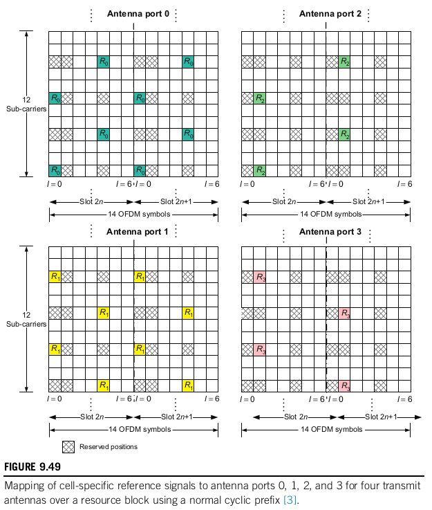
To the pattern shown above, a frequency offset that consists of the PCI (physical cell ID) modulo 6 subcarriers is applied. This is done so that the reference signals of cells having different PCIs use different subcarriers, so as to prevent interference (especially those cells in the same group, since their PCI modulo 3 is different).
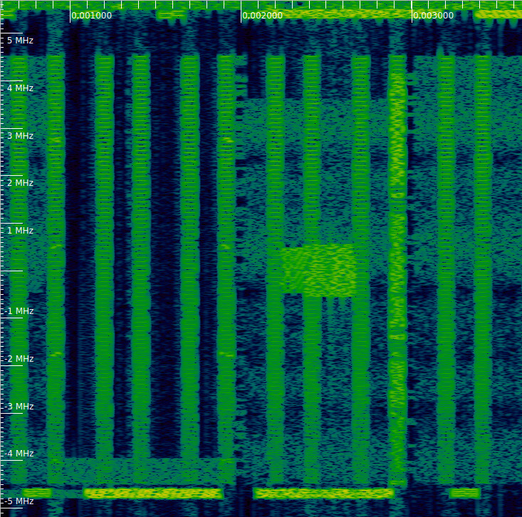
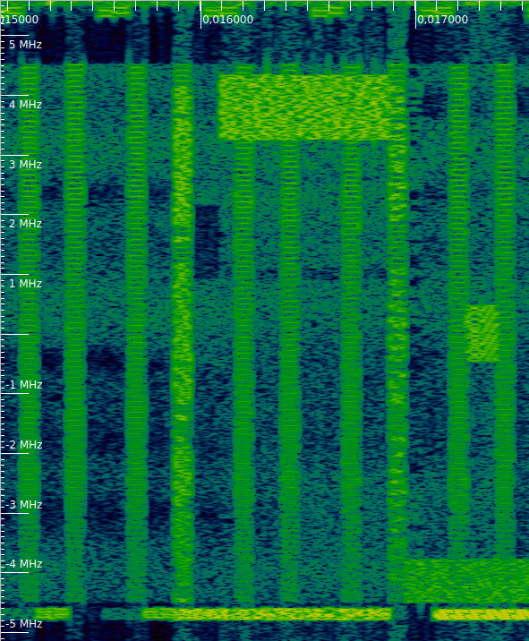
In the waterfall of our recording, we can clearly see the CRS transmissions. They last one symbol and occupy the whole bandwidth of the cell. We can also see the PSS, SSS and PBCH, as we remarked in the previous post. These indicate us where the subframes start. Thus, we can see that the first and fifth symbol of each slot are used for transmission of the CRS. This means that the cell does not use four antenna ports, since their corresponding CRS would be transmitted on the second symbol of each slot.
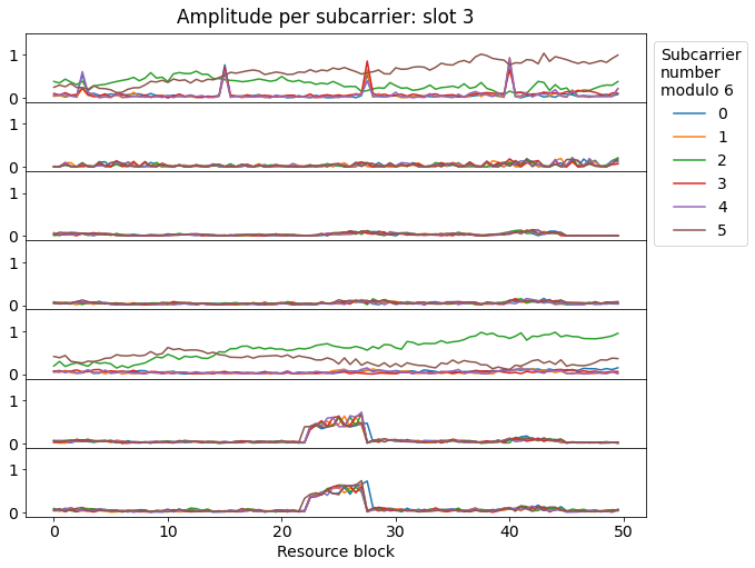
To look at the CRS in more detail, we use the synchronization parameters that we found in the previous post (symbol time offset and carrier frequency offset) and perform OFDM demodulation of the the symbols in the recording. Now we can plot, for each OFDM symbol, the amplitude of each subcarrier, grouping them by their index modulo 6. This will show us which subcarriers are being used for CRS transmission, which is hard to tell in the waterfall.
This is the plot corresponding to the 7 symbols in slot 0, which is the first full slot in the recording (the slot number used here is arbitary, and unrelated to the radio frame). We see that subcarriers with indexes congruent with 2 and 5 modulo 6 are being used in the first and fifth symbols. The cell is quiet in all the other resource elements. This indicates that the cell uses two antenna ports for the transmission of the CRS. The amplitude of the recording has been normalized so that the strongest subcarriers have an amplitude of approximately one.
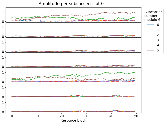
The PCI of this cell is 380, which modulo 6 gives 2. This means that the green trace in the the first symbol corresponds to \(R_0\), and the brown trace corresponds to \(R_1\). In the fifth symbol \(R_0\) and \(R_1\) switch positions. We can notice this by observing the patterns of the amplitude versus frequency.
It is interesting to look at this kind of plot for the subsequent slots. In the next slot we can see that there are some additional subcarriers being used in four resource blocks in the first symbol. These correspond to the PCFICH (physical control format indicator channel), which we will look at later in more detail. The PCFICH transmissions happen at the start of each subframe. Looking closely at the waterfall, we can also spot them there.
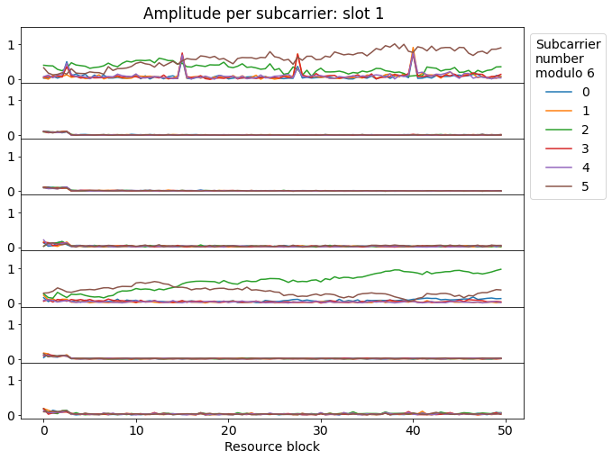
Additionally, we can see that the lower resource blocks are being used by another (much weaker) cell, while the remaining of the spectrum is clear. This can also be seen in the waterfall.
The next slot looks very similar to slot 0, except for the activity of the weaker cell in the background.

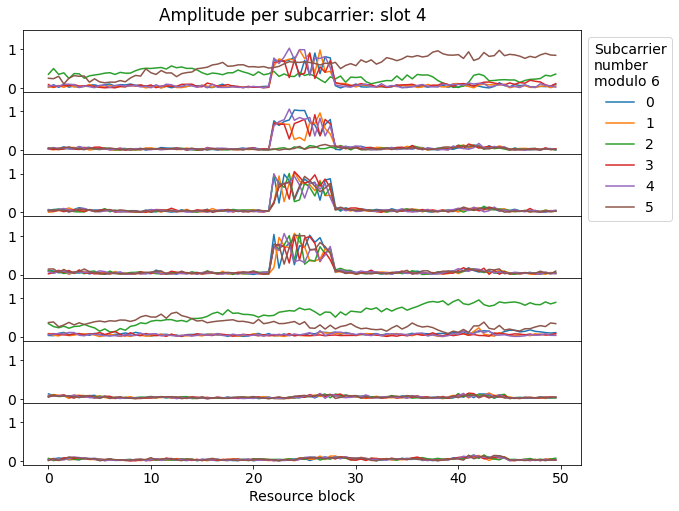
Now we arrive to the slot where the synchronization signals are transmitted. We can see them in the last two symbols, occupying the central 6 resource blocks (except for a few subcarriers at the edges, left empty as a guard band).
In the next slot we have the PBCH transmission, which occupies the first four symbols. When a UE is attempting to decode the PBCH, it does not necessarily know the number of antenna ports in use for the CRS. Therefore, the PBCH is always transmitted assuming that all four ports are used, in the sense that the PBCH avoids the resource elements assigned to each of the four ports. We can see this in the second symbol, where subcarriers with indexes congruent with 2 and 5 modulo 6 are quiet. These would correspond to \(R_3\) and \(R_4\). In contrast, in the third and fourth symbols the PBCH occupies all the subcarriers in the 6 central resource blocks, since no CRS is transmitted these symbols.
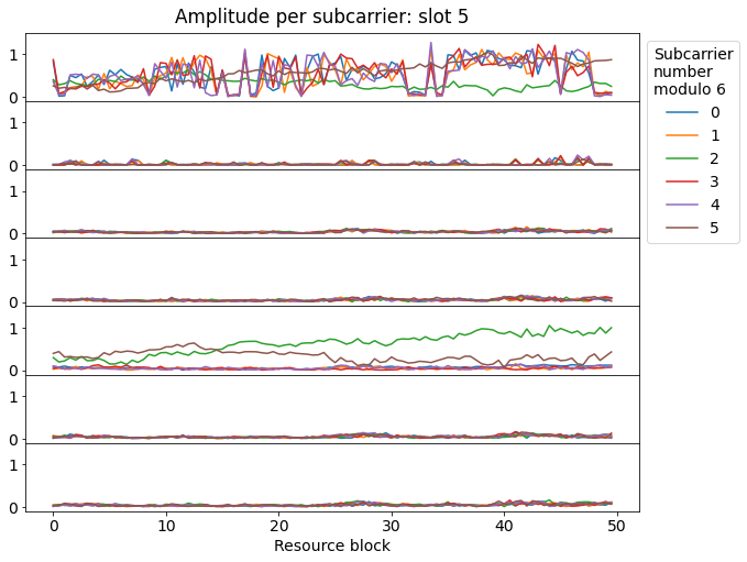
Finally, in the next slot we see that in the first symbol there are many active subcarriers, besides those corresponding to the CRS and the PCFICH. These correspond to the PHICH (physical hybrid-ARQ indicator channel) and PDCCH (physical downlink control channel), which are sometimes transmitted in the first or first two symbols of a subframe. Looking carefully at the waterfall, the presence of the PDCCH can also be spotted there, since the corresponding symbol looks stronger and has a slightly different texture than when only the CRS and PCFICH are transmitted.
Channel estimation
The first step in channel estimation is to wipe off the modulation of the CRS. The subcarriers used by the CRS in each OFDM symbol are modulated in QPSK using a pseudorandom sequence. The sequence depends, among other things, on the PCI, so different cells use different sequences with low cross-correlation. This gives an additional degree of protection against inter-cell interference.
As many other pseudorandom constructions in LTE, the CRS uses the sequence described in Section 7.2 of 3GPP TS 36.211. This defines a family of Gold codes of length \(2^{31}-1\). Recall that such a family is composed by the sequences obtained by XORing two M-sequences in all their possible relative circular shifts. In the case of LTE, the code in the family is selected using a seed \(c_{init}\) that depends on the intended application, and a subsequence of the appropriate length is extracted from the Gold code.
For the CRS, the value of \(c_{init}\) depends on the PCI, on the slot number within the radio frame, and on the symbol number within the slot. Therefore, the sequence used by each cell keeps changing in each OFDM symbol, but the pattern repeats every radio frame.
Another interesting aspect of the pseudorandom generation of the CRS is that regardless of the bandwidth of the cell, we always generate a sequence that is long enough to construct the CRS for 110 resource blocks (which is slightly wider than the widest possible bandwidth of 100 resource blocks, used by 20 MHz cells). Then a subsequence whose length matches the bandwidth of the cell is extracted from the middle of this longer sequence. The consequence of this construction is that the sequence that gets assigned to some particular resource blocks does not depend on the cell bandwidth (as long as those resource blocks are present in the cell bandwidth).
This property can be used by the UEs to help them demodulate the PBCH. When a UE first demodulates the PBCH, it does not necessarily know the cell bandwidth. Regardless of this, it can construct the CRS corresponding to the 6 central resource blocks and use them to equalize the PBCH.
Once we generate the pseudorandom QPSK sequences, we can wipe off them from the received CRS symbols, and look at the resulting amplitude and phase, which indicate the amplitude and phase of the channel.
The figures below show the amplitude and phase of the CRS of each of the two antenna ports. The first four symbols containing CRS are shown with traces of different colours. We see that there is a very consistent behaviour over time. Even the phase does not rotate, since we have estimated the carrier frequency offset quite precisely before OFDM demodulation.
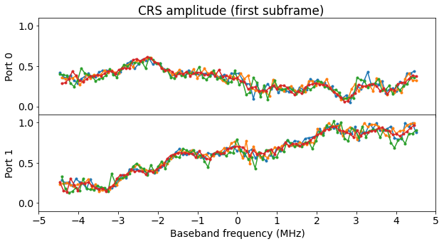
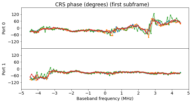
I am intrigued by the non flatness of these channel responses. As I attempted to record the cell signals with a line-of-sight path (see the previous post for a description of the recording set up), I would have expected a much flatter channel. In contrast, we see that the amplitudes of the two ports are by no means flat, and there are even frequencies at which there is almost a null, with its corresponding jump in phase. These are around 3 MHz for port 0 and -3.5 MHz for port 1.
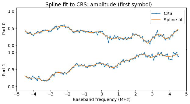
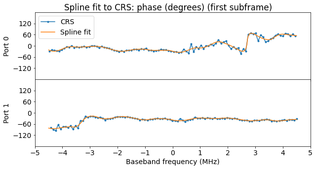
To construct a channel estimation from the CRS, I have decided to perform a least squares fit of a cubic spline to the CRS complex amplitude. Each of the segments of the spline occupies 5 of the 50 resource blocks used by the cell. I think this gives a good balance between over-fitting and frequency resolution. Also, having the full cell bandwidth being evenly divided into spline segments of the same size simplifies things. Since there are 10 spline segments in total, the spline is defined by 22 complex coefficients.
The figures below show the spline fit corresponding to the first symbol.
To obtain the channel estimation for any symbol in which CRS are not transmitted, the splines of the two CRS adjacent in time to this symbol are linearly interpolated. The interpolation can be applied directly to the coefficients defining the spline, since the spline depends linearly on its coefficients.
There is an important point regarding this interpolation in time and the effect of the sampling frequency offset. In the previous post we estimated a sampling frequency offset of around 1.5 ppm. In OFDM demodulation, we took the sampling frequency offset into account by computing the sample in which each OFDM symbol would start, and rounding that to the nearest integer sample. This causes symbol time offset errors as large as 0.5 samples (at 30.72 Msps), and jumps in the error on the order of 1 sample when the direction in which rounding is done changes.
When considering the full 10 MHz bandwidth of the cell, these jumps are excessive. They would cause a jump in phase in the order of 53 degrees for the outer subcarriers. This messes up our time interpolation of the channel estimation. To avoid these jumps, the fractional sample error is corrected during OFDM demodulation by applying a suitable phase versus frequency slope to the subcarriers.
Transmit diversity
When the cell uses two ports for the CRS, as is the case here, several transmissions, including the PBCH can be done with transmit diversity. This uses an Alamouti code to transmit the data on two antenna ports. In this way, a UE with a single antenna can recover the data even if the channel for one of the base station antenna ports is faded.
Transmit diversity is done by precoding the data before transmission. The symbols to be transmitted are grouped in pairs, and the subcarriers to be used are also grouped in pairs of adjacent subcarriers. Each pair of symbols \(x_0, x_1\) is mapped into two pairs of complex values \(y_0^p, y_1^p\), \(p = 0, 1\) that are transmitted simultaneously over the same pair of subcarriers in the two ports \(p = 0, 1\). The mapping is\[\begin{split}y_0^0 &= x_0,\\y_1^0 &= x_1,\\y_0^1 &= -\overline{x_1},\\y_1^1 &= \overline{x_0}.\end{split}\]
If we denote by \(h_j^p\) the channel response for subcarrier \(j = 0, 1\) and base station antenna port \(p = 0, 1\), we see that the UE receives the symbols\[\begin{split}z_0 &= h_0^0 y_0^0 + h_0^1 y_0^1 = h_0^0 x_0 – h_0^1 \overline{x_1},\\z_1 &= h_1^0 y_1^0 + h_1^1 y_1^1 = h_1^0 x_1 + h_1^1 \overline{x_0}.\end{split}\]Let us assume that \(h_0^p = h_1^p\) for each \(p\), which is a reasonable assumption, since the two subcarriers are adjacent in frequency. Denoting \(h^p = h_0^p = h_1^p\), we see that the UE can recover the symbols \(x_j\) by computing\[\begin{split}\frac{\overline{h^0}z_0 + h^1 \overline{z_1}}{|h^0|^2 + |h^1|^2} &= x_0,\\\frac{-h^1\overline{z_0} + \overline{h^0}z_1}{|h^0|^2 + |h^1|^2} &= x_1.\end{split}\]In the general case where \(h_0^p\approx h_1^p\), the above equalities are only approximate equalities, but they are still good enough to recover the symbols \(x_j\).
It is easy to check that when the UE computes \(x_j\) from \(z_j\) using the formulas above, assuming that \(z_j\) have the same noise variance \(\sigma^2\) and that their noise is uncorrelated, then the noise variance of \(x_j\) is \(\sigma^2/(|h^0|^2 + |h^1|^2)\). This shows that this transmit diversity scheme really manages to combine all the received power from both transmit antennas in the UE.
Section 6.3.4.3 in TS 36.211 includes an additional factor \(1/\sqrt{2}\) in the precoding formulas that define \(y_j^p\) in terms of \(x_j\). However, when handling the transmit diversity I haven’t needed to account for this factor. I don’t know if there is another factor I’ve missed that is cancelling this one.
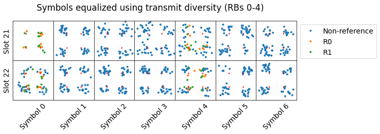
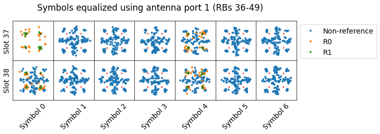
The PDSCH (physical downlink shared channel) transmission shown in the top of the waterfall below serves well to illustrate transmit diversity. For the higher frequencies of the cell, the signal from port 1 is much stronger than the signal of port 0. This means that in the received symbols \(z_j = h_j^0 y_j^0 + h_j^1 y_j^1\) the contribution from \(y_j^1\) will dominate.
In fact, we can show this by equalizing the symbols of this PDSCH transmission using only the channel for port 1. These are shown in blue in the figure below. The symbols for the CRS for port 0 and port 1 are shown in orange and green respectively. These are equalized with the channel for the corresponding port. The symbols corresponding to \(R_1\) are much less noisier than those for \(R_0\), since port 1 has much more SNR.
Looking at the figure attentively, we can see that the resulting constellation for the data symbols looks like four a small QPSK constellations, each centred on the nominal locations of the usual QPSK constellation.

Indeed, here we are looking at \(z_j/h_j^1 = (h_j^0/h_j^1) y_j^0 + y_j^1\). Each of the terms \(y_j^p\) follows a QPSK constellation, and the factor \(|h_j^0/h_j^1|\) is much smaller than one. Thus, we are mainly seeing \(y_j^1\), and the term \(y_j^0\) acts as a perturbation.
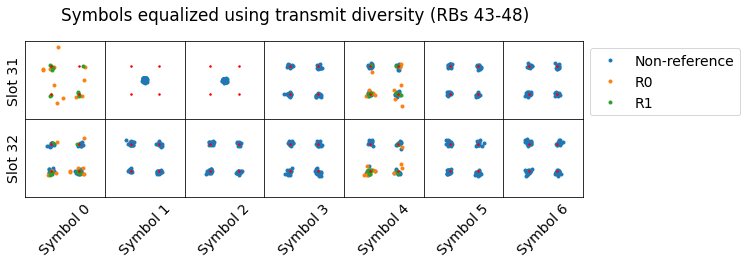
If we instead perform equalization using the transmit diversity formulas described above, we obtain a tight QPSK constellation. We have combined the perturbation from \(y_j^0\) and the main component \(y_j^1\) to recover the sum of the powers from both transmit antennas.
In the case when the amplitudes of the channels for both ports are similar, it is much more difficult to recognise the shape of the constellation if we only use the channel of one port for equalization, so using the proper transmit diversity equalization is essential for correct demodulation.
PBCH demodulation
The PBCH (physical broadcast channel) is transmitted using the 6 central resource blocks, in the first 4 symbols of the second slot in each radio frame. This cell uses transmit diversity for the PBCH. The figure below shows the equalized PBCH symbols and the adjacent CRS symbols.
To extract the PBCH symbols we need to remember that the locations in the second symbol that would correspond to the CRS for ports 2 and 3 are left unused.
The figure below shows the PBCH symbols during all the one second recording. All the symbols corresponding to a PBCH transmission are shown in the same square. There are a total of 100 PBCH transmissions shown in a 10×10 grid that should be read from left to right. Since the PBCH is transmitted every 10 ms, this amounts to one second of data.

The lower SNR in some of the PBCH transmissions is caused by interference from other cells in the background. The waterfall below shows the last 9 PBCH transmissions. I have marked each of them with a red tick, but the image is probably better seen in full screen (by clicking on it). There are 3 transmissions in the bottom row of the figure above that have less SNR. These correspond to the time interval between 0.92 and 0.95 seconds, where there is a stronger transmission from another cell.

PCFICH demodulation
The PCFICH (physical control format indicator channel) is always transmitted in the first symbol of each subframe. It carriers the CFI, which is an integer \(k\) between 1 and 3 that defines how many symbols of a subframe are used for control information. The first \(k\) symbols of the subframe will be used for the PHICH and PDCCH, while the remaining \(14 – k\) symbols will be used for the PDSCH (physical downlink shared channel), which carries the user data.
As other control channels, the PCFICH is transmitted in REGs (resource element groups). These are groups of 4 resource elements which occupy the 4 subcarriers not allocated to CRS in a set of 6 subcarriers aligned to the resource block grid (i.e., one half of the 12-subcarrier resource block).
The PCFICH uses 4 REGs, which are regularly spaced in frequency across all the cell bandwidth in order to provide frequency diversity. Additionally, the location of these REGs depends on the PCI to prevent interference between different cells.
A REG is identified by the subcarrier index of the lower subcarrier in the group of 6 subcarriers in which the REG is placed. This index should be a multiple of 6. For the PCFICH, the 4 REGs used correspond to the indices \(\overline{k} + 6\lfloor j N^{DL}_{RB} / 2\rfloor\), for \(j = 0, 1, 2, 3\). Here \(N^{DL}_{RB}\) is the number of resource blocks in the downlink (50 for a 10 MHz cell) and the offset \(\overline{k}\) is given by \(\overline{k} = 6(N_{ID}^{cell} \mod 2 N^{DL}_{RB})\).
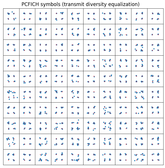
The PCFICH uses the same transmission scheme as the PBCH, so in this case it uses transmit diversity on ports 0 and 1. The figure below shows the equalized symbols corresponding to the first 100 PCFICH transmissions, as a 10×10 grid. Each square in the grid contains the 16 QPSK symbols that form a PCFICH transmission. We can see that some of the symbols are a bit noisy. I haven’t looked at the cause in detail.
The 32 bits carried by the PCFICH are scrambled with a pseudorandom sequence that depends on the PCI and the slot number with the radio frame. The PCI value is encoded into a 32 bit code word as indicated in the following table in 3GPP TS 36.212.
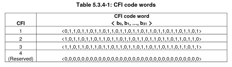
Using this table, we can decode the CFI after descrambling. Here I am using hard decision on the QPSK symbols and choosing the codeword that has the minimum Hamming distance. A soft decision scheme would be better, but with this good SNR it is not necessary. The number of bit errors in the hard decision decoding is zero almost always, and just one on a few occasions.
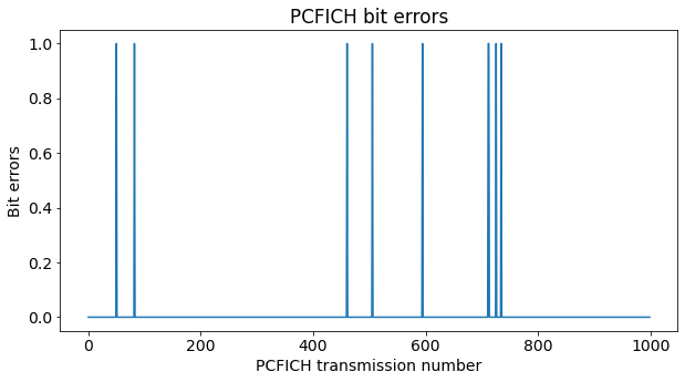
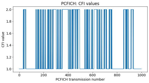
The decoded CFI values are shown below. We see that the CFI alternates between 1 and 2, and is never 3.
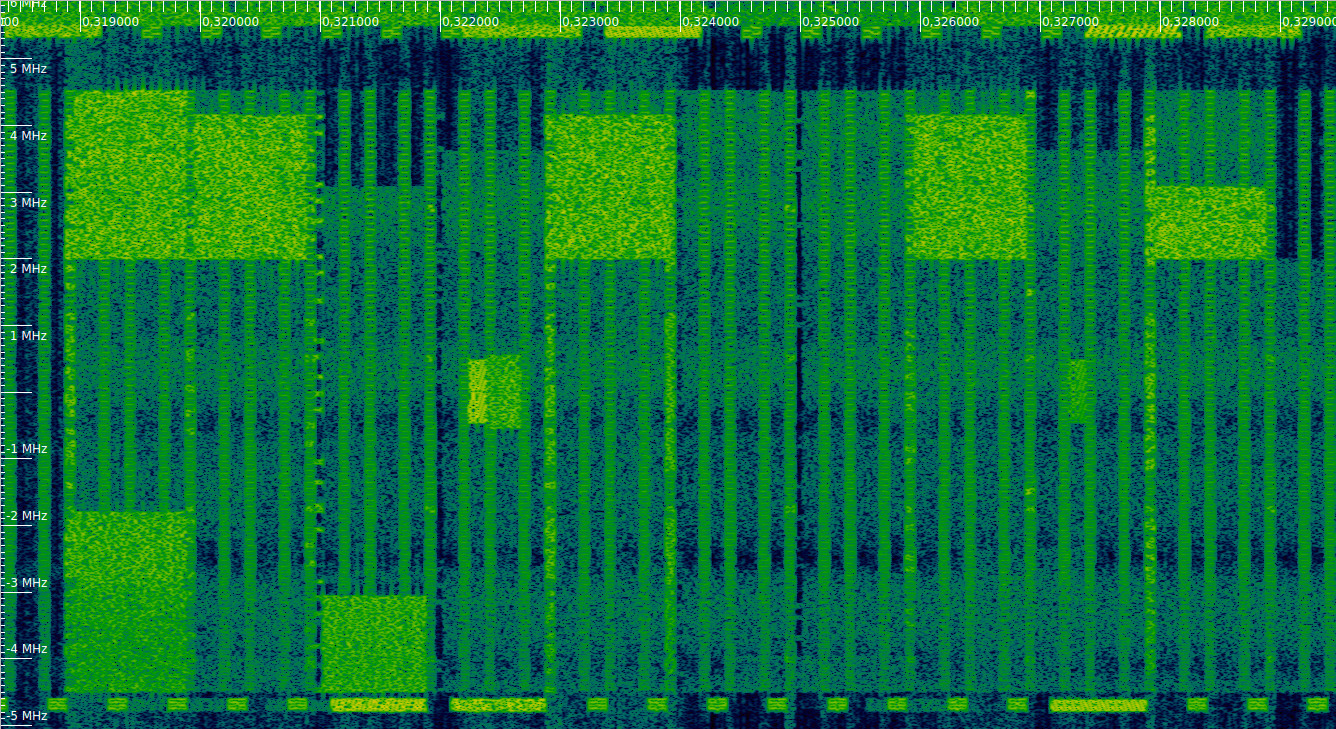
It is possible to guess the CFI value by looking at the waterfall. The waterfall below shows 3 full subframes. The first of them, which contains the PSS and SSS, has a CFI of 1, since the second symbol is empty (except for a PDSCH transmission using the lower resource blocks). The next subframe, in the middle of the waterfall, has a CFI value of 2. We see that the second symbol contains many REGs that are used for the PDCCH. Finally, the next subframe uses a CFI of 1 and only has CRS.
PDSCH detection
The PDSCH (physical downlink shared channel) is the channel that carriers the user data. Each PDSCH transmission occupies the last \(14 – k\) symbols of a subframe, where \(k\) is the CFI value for that subframe. The frequency allocation for a PDSCH transmission is always a set of 12-subcarrier resource blocks (often contiguous, but not necessarily, due to a feature called VRBs). The size of the frequency allocation depends on the size of the codeword that needs to be sent. Data can be sent to different UEs simultaneously by using different frequency allocations for each of them (the LTE downlink uses OFDMA). The PDSCH can use QPSK, 16QAM or 64QAM.
The figure below shows 7 different PDSCH transmissions. Most of them happen in subframes with a CFI of 1, but we can see that the third subframe has a CFI of 2.
To detect the time-frequency allocations in which the PDSCH is transmitted, we can compute the downlink signal power for each time-frequency bin of size one resource block times one subframe. Before doing this, we blank the channels that are not PDSCH, using their known locations. We can blank the PCFICH, the CRS, the PSS and SSS, the PBCH, and also the first symbols in each subframe as indicated by the CFI, since those belong to control channels (if we do this, it is not really necessary to blank the PCFICH, since it is transmitted in the first symbol of each subframe, which is always allocated to control channels).
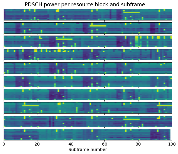
The figure below shows the results of the power measurements of the PDSCH per resource block and subframe. Each line of the plot encompasses 100 subframes (100 ms), so the 10 lines show the one second of data. We can see that most of the time the cell is idle, but there are occasional PDSCH transmissions that occupy only a fraction of the bandwidth. There are also a few long transmissions which last 10 subframes and repeat 3 times with a separation of 80 ms. We will look at these in more detail later.
By doing a threshold selection of the data plotted above, we can determine the PDSCH allocations. This can be used to demodulate each of them. There are a total of 466 detected PDSCH allocations, so we won’t look at all of them in this post.
PDSCH demodulation
Using the allocations detected in the previous step, we can demodulate each of the PDSCH transmissions. By default, I’m using transmit diversity equalization. However, this doesn’t seem to work well for many of the transmissions. For instance, this is the first PDSCH transmission in the recording.
And this is the next one.

Neither of them shows a clean constellation as we would expect given the SNR of the signal. PDSCH transmissions can also be sent using other transmission schemes that are equalized with UE-specific reference signals. In this post I am not considering UE-specific signals, since I haven’t found a way of handling them without decoding the downlink scheduling assignments in the PDCCH.
In contrast, there are other transmissions that equalize really well using transmit diversity. This is the third PDSCH allocation in the recording. Note that symbol 1 and symbol 2 in the first slot do not carry data, despite the fact that the CFI is 1. We will come back to this later.
There are other transmissions that look like a complete mess when we equalize them using transmit diversity. For instance, these two, which happen simultaneously using resource blocks at the two edges of the cell bandwidth.

If we equalize the second of these two transmissions using the channel for port 1 only, we can see a constellation that looks like the four QPSK points plus a cross along the real and imaginary axes. I haven’t given much thought to why this pattern emerges, but it could give some clues about how the data is precoded and transmitted.
More figures showing PDSCH demodulation can be found in the Jupyter the Jupyter notebook.
Transmissions for BL/CE UEs
I have noticed that there are some PDSCH transmissions that always start in the fourth symbol of the subframe, regardless of the CFI value. I think these are transmissions for BL/CE UEs (also known as LTE-M1). I don’t know a lot about BL/CE, but the characteristics of these transmissions matches some of the constraints used by BL/CE. These are UEs that are limited to 1.4 MHz bandwidth and half-duplex. Therefore, their PDSCH transmissions are scheduled in some particular sets of 6 contiguous resource blocks known as narrowbands, the UEs do not use the control signals that are spread over all the cell bandwidth (such as the PDCCH), and there are guard intervals for TX/RX switch and retuning.
Interestingly these transmissions are the ones that equalize really well using transmit diversity. This suggests that maybe this cell is only using transmit diversity on ports 0 and 1 for BL/CE UEs, and other UEs use other transmit schemes involving UE-specific reference signals.
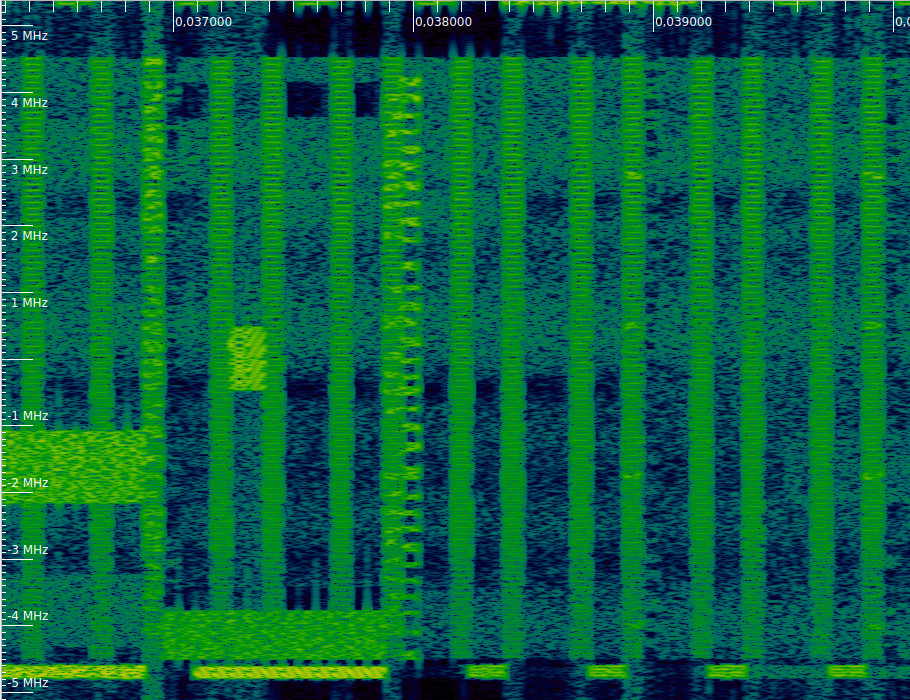
The waterfall below shows several examples of this kind of transmissions. I have marked one of them in red, and there is also a series of transmissions between 1 and 2 MHz. Note that all of them leave an unused gap of two symbols between the symbol occupied by the CRS and the first PDSCH symbol.
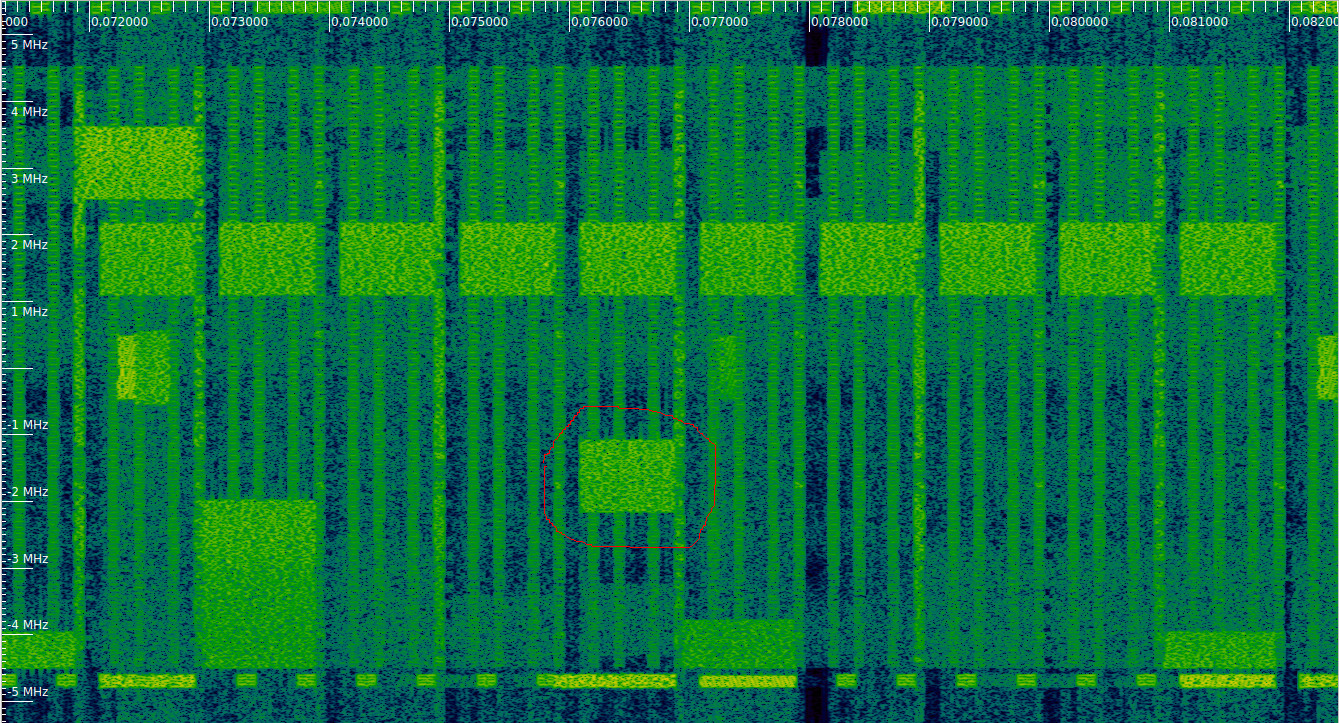
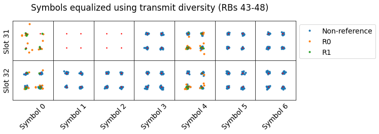
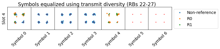
Additionally, all of these transmissions are 6 resource blocks wide. The sets of resources blocks they occupy is precisely one of the BL/CE narrowbands for a 10 MHz cell (as listed in this table). We see RBs 13-18, 31-36 (this is where the series of 10 contiguous transmissions happens), and 43-48 being used in this way.
The series of 10 transmissions between 1 and 2 MHz that appears in the waterfall above corresponds to the long transmissions that we saw in the figure that shows the PDSCH power. I think this is some control data (maybe the SIB) for BL/CE, but I haven’t been able to identify which just by looking at the timing.
Code and data
The recording used in this post is the same that I used in the previous post. It is the LTE_downlink_806MHz_2022-04-09_30720ksps SigMF recording in this LTE recordings folder. The calculations and plots have been done in this Jupyter notebook.
3 comments