This is a long overdue post. In 2022, I wrote a series of posts about LTE as I studied its physical layer to understand it better. In the last post, I decoded the PDCCH (physical downlink control channel), which contains control information about each PDSCH (physical downlink shared channel) transmission. I found that, in the recording that I was using, some PDSCH transmissions used Transmission Mode 4 (TM4), which stands for closed-loop spatial multiplexing. For an eNB with two antenna ports (which is what I recorded), this transmission mode sends either one or two codewords simultaneously over the two ports by using a precoding matrix that is chosen from a list that contains a few options. The choice is done by means of channel-state information from the UE (hence the “closed-loop” in the name).
In the post I found a transmission where only one codeword was transmitted. It used the precoding matrix \([1, i]^T/\sqrt{2}\). This basically means that a 90º phase offset is applied to the two antenna ports as they simultaneously transmit the same data. I mentioned that this was the reason why I obtained bad results when I tried to equalize this PDSCH transmission using transmit diversity in another previous post, and that in a future post I would show how to equalize this transmission correctly. I have realized that I never wrote this post, so now it is as good a time as any.
Downlink power allocation
Before beginning with TM4, I need to go back to the post where I spoke about transmit diversity. There, I mentioned that there was a \(1/{\sqrt{2}}\) factor in TS 36.211 that I couldn’t account for. The formula for transmit diversity precoding over two antenna ports is shown here (this is taken from Section 6.3.4.3 in TS 36.211).
However, the formula I used for equalization was the same one but without the \(1/\sqrt{2}\) factor. If I included this factor, I obtained a QPSK constellation with amplitude \(\sqrt{2}\) rather than one. I couldn’t find anything in the 3GPP documents that explained why this factor was being cancelled. This is relevant for TM4, because the precoding matrices also have this \(1/\sqrt{2}\) factor.
Doing more research about this, I have realized that I was missing an important piece of the puzzle: downlink power allocation. It turns out that in LTE the power used by each resource element of the PDSCH and other downlink signals can be different from the power of the resource elements used by the CRS (cell-specific reference signal). The power levels are defined relative to the CRS resource elements, and configured by the higher-layers. A UE needs to know these power ratios in order to perform equalization correctly. Knowing the amplitude (or power) relation between a signal such as the PDSCH and the CRS is not terribly important for QPSK, because failure to use the correct ratio only scales the constellation. However, it is critical for QAM constellations.
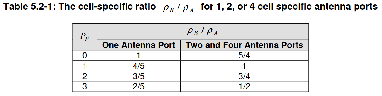
The details of how this works are in Section 5.2 in TS 36.213. This section is quite confusing to read, because there are many special cases and higher-layer parameters mentioned. Some summaries of this information are the one by ShareTechnote, this one by Smart Telecom Edu, and a post in the Huawei forums. Briefly speaking, for the PDSCH there are two quantities \(\rho_A\) and \(\rho_B\) that define the power ratio between PDSCH resource elements and CRS resource elements. The value \(\rho_A\) is used for resource elements in symbols in which there are no CRS (symbols 1, 2, 3, 5, 6 for two antenna ports and normal cyclic prefix), and \(\rho_B\) is used for resource elements in symbols in which there are CRS (symbols 0 and 4 for two antenna ports and normal cyclic prefix). There is much flexibility to set \(\rho_A\), and it can even by set differently per UE. However, the value of \(\rho_B\) is determined from \(\rho_A\) by the quotient \(\rho_B/\rho_A\), which has a fixed value given by a parameter \(P_B\) transmitted in the SIB2, according to this table in TS 36.213.
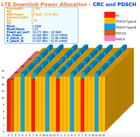
The missing \(1/\sqrt{2}\) factor that I was observing can be explained if for this particular recording \(\rho_A = \rho_B = 2\). Most of the examples in these summaries have \(\rho_A < 1\), meaning that less power is allocated to the PDSCH resource elements than to the CRS resource elements. They mention that it is important to allocate higher power to the CRS because the reference signals need to have higher SNR for good equalization, but there are also some examples with \(\rho_A > 1\), such as the following, taken from the video that accompanies the Smart Telecom Edu post.
Something that I haven’t seen mentioned when discussing downlink power allocation is that the precoding matrices for two antenna ports all have the property that if the input is a QPSK constellation with power one (either one or two layers of this), then the total power over both antenna ports has an expected value of one. This happens thanks to the \(1/\sqrt{2}\) and \(1/2\) factors in the matrices in the following table taken from TS 36.211, and also for transmit diversity precoding. Technically speaking, these factors make the Hilbert-Schmidt norm of these matrices equal to one, which is what is required to obtain this kind of power normalization.
However, in some situations it might be more reasonable to consider what happens with the power of each antenna port individually, and normalize things so that the power of each port has expected value one (and hence the total power over both ports has an expected value of 2 for these two-port transmissions). For instance, if each antenna port has a separate power amplifier, this can be a good point of view (although if we are considering the eNB for spectrum management, then total power over all ports is a better metric). This normalization is achieved by setting \(\rho_A = \rho_B = 2\), and in a sense this is a rather natural choice, as it makes all the resource elements in each port have the same power. It is true that, for each port, the resource elements occupied by the CRS of the other port are muted, and hence the symbols containing CRS resource elements have 5/6 of the power of the other symbols. If we want to have the same power in all the symbols by increasing the power of PDSCH resource elements in symbols containing CRS, then that is what the setting \(P_B = 0\), which gives \(\rho_B/\rho_A = 5/4\) is for.
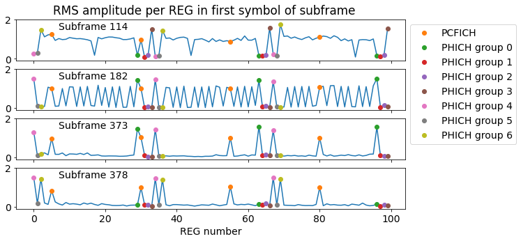
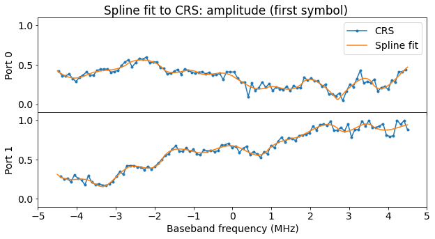
Another interesting aspect of power allocation in the recording I have been using is that the PHICH (physical hybrid-ARQ indicator channel) has twice more power than the other physical downlink channels, such as the PCFICH, the PDCCH and the PBCH. All these channels use transmit diversity, but when equalized in the same way, the constellations for the PCFICH, PDCCH and PBCH have amplitude 1 but the constellation for the PHICH has amplitude \(\sqrt{2}\) (so it has twice as much power). I mentioned this in my post about the PHICH. The higher power allocation for the PHICH is clear even in this plot, which shows the RMS amplitude in each REG in the first symbol of some subframes. We can see that the PHICH REGs that are active have a larger amplitude than the PCFICH REGs and the REGs occupied by the PDCCH.
Looking into how downlink power allocation is defined by the standard, I haven’t found an explanation for why the PHICH can be set to a higher power than the other channels. I think that given that the PHICH uses a BPSK constellation and doesn’t use any FEC that requires knowledge of the amplitude for decoding (which is what happens with the FEC decoders that need LLRs), the UE doesn’t really care about how much power is allocated to the PHICH. Probably, in practice the eNB is free to set the PHICH power level as it desires, without indicating this choice to the UEs.
TM4 with one codeword
DCI and precoding matrix
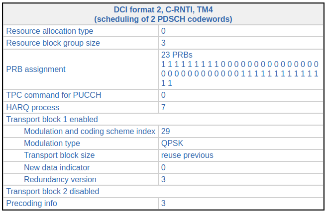
In the post about the PDCCH, I showed that one of the PDSCH transmissions had the following DCI in the PDCCH. This is a TM4 transmission, but only one transport block is active. This means that there is only one codeword (and one layer) used in the spatial multiplexing precoding.
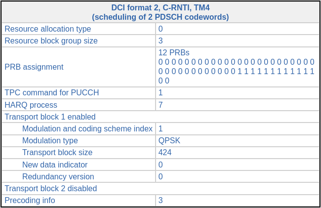
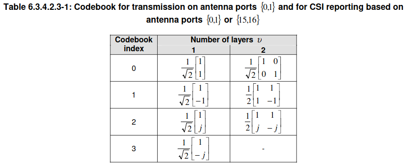
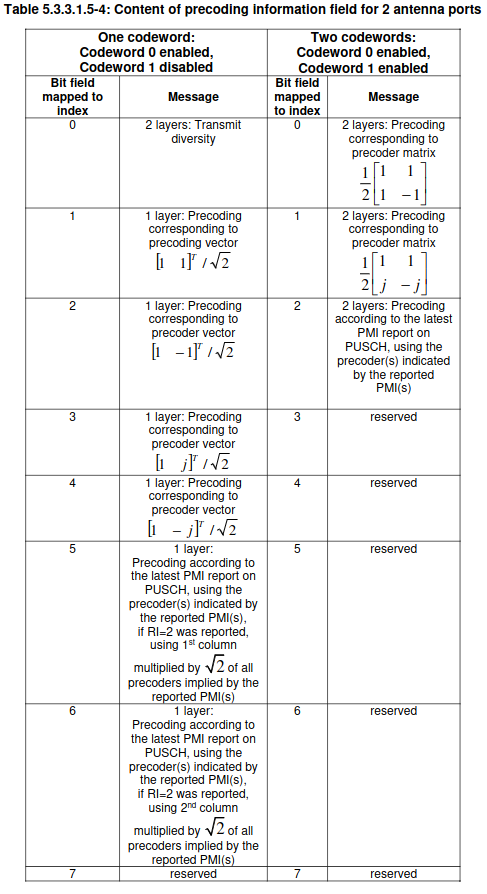
The precoding information in the DCI is 3. This indicates which precoding matrix is used, but it doesn’t refer to the codebook index of the TS 36.211 Table 6.3.4.2.3-1 shown above. The table that needs to be used to interpret this DCI field is Table 5.3.3.1.5-4 in TS 36.212, reproduced here. The precoding matrix corresponding to the value 3 is \([1, i]^T/\sqrt{2}\).
Equalization and SNR analysis
In general, when a single codeword is transmitted with a precoding matrix \([a_0, a_1]^T\), this means that for each resource element the output of antenna port \(p\) is\[y_p = a_p x,\]where \(x\) is the symbol in the codeword that is mapped to this resource element. Assuming that the receiver has a single antenna and denoting by \(h_p\) the channel response between antenna port \(p\) of the transmitter and the receiver antenna, we see that (ignoring noise), the received receives the symbol\[z = h_0 y_0 + h_1 y_1 = (a_0 h_0 + a_1 h_1) x.\]Therefore, it can recover \(x\) as\[x = \frac{z}{a_0 h_0 + a_1 h_1}.\]The values of \(a_p\) are known, and \(h_p\) are estimated using the CRS.
If the received symbol \(z\) has noise variance \(\sigma^2\), then the noise variance of \(x\) is \(\sigma^2 / |a_0 h_0 + a_1 h_1|^2\). The noise variance for a transmission over a single antenna port \(p\) would be \(\sigma^2 / |h_p|^2\), and as we saw in the post about transmit diversity, the noise variance for transmit diversity would be \(2 \sigma^2 / (|h_0|^2 + |h_1|^2)\) (here I am assuming that we have the \(1/\sqrt{2}\) factor in the precoding formulas, so that the total transmitted power over all ports is the same in the three cases; for the TM precoding matrix this condition is \(|a_0|^2 + |a_1|^2 = 1\)).
Comparing transmit diversity and transmission over a single port under this condition shows that if we know which port \(p\) has maximum channel response \(|h_p|\), then it is advantageous to transmit only over this port. However, if we don’t know which port \(p\) is better, then transmit diversity is a good option because it gives an SNR which is better or equal than -3 dB compared to single port transmission over the best port. This explains why transmit diversity is so useful for transmissions in which it is not possible to select the best port \(p\) because either we don’t have CSI (channel state information) from the UE or because the transmission is addressed to several UEs (as is the case with the control channels).
If we now consider single-codeword TM4, assuming that we had perfect CSI and that we could choose any precoding matrix, according to Cauchy-Schwarz the best that can be done is to choose \(a_p = \overline{h_p}/\sqrt{|h_0|^2 + |h_1|^2}\). This gives a noise variance of \(\sigma^2 / (|h_0|^2 + |h_1|^2)\). This is exactly 3 dB better than transmit diversity, and always better than single-port transmission. However, in reality the choice of precoding matrix is limited to one of the form \([1, i^k]^T/\sqrt{2}\) for \(k = 0, 1, 2, 3\). The optimal choice with this limitation depends on the value of \(\alpha = \arg(h_0 \overline{h_1})\). Namely, it is\[k = \left\lfloor \frac{2\alpha}{\pi} + \frac{1}{2}\right\rfloor \mod 4.\]Intuitively speaking, this choice is the one that aligns the phases of \(a_0 h_0\) and \(a_1 h_1\) in the best possible way. In the worst case, the phase of these two numbers will differ by \(\pi/4\), because the choices for \(a_1\) are spaced \(\pi/2\) apart in phase. Therefore, we always have\[|a_0 h_0 + a_1 h_1|^2 \geq \frac{1}{2}\left(|h_0|^2 + |h_1|^2 + \sqrt{2}|h_0||h_1|\right).\]
We see that single-codeword TM4 with the appropriate precoding matrix always gives more SNR than transmit diversity. In the special case when \(|h_0| = |h_1|\), single-codeword TM4 gives at least a factor of \(1 + \sqrt{2}/2\) more SNR than transmit diversity. This is 2.32 dB, which is not far from the ideal 3 dB difference that can be achieved with an arbitrary precoding matrix. However, when \(|h_0| \ll |h_1|\) or vice versa, the above equation shows that the improvement of single-codeword TM4 over transmit diversity is very small.
Single-codeword TM4 as transmit beamforming
It is possible to interpret single-codeword TM4 as a form of transmit beamforming. The effect of the precoding matrix is to transmit the same signal over both ports, but using a phase offset between the ports that must be an integer multiple of \(\pi/4\) (or 90 degrees). From the possible 4 “beams” to choose from, the one which gives better SNR because it aligns better the phases of the signals at the receiver is the one that is used.
Interestingly, it seems that many 2-port eNBs use cross-polarized antennas in an X pattern. One of the antenna ports is the +45 deg polarization, and the other port is the -45 deg polarization. For instance, the following figure from a Rohde & Schwarz whitepaper on LTE TMs shows typical eNB antenna configurations. The 2-port configuration is the one on the left. The antenna elements in red form one port, and the antenna elements in blue form the other port.
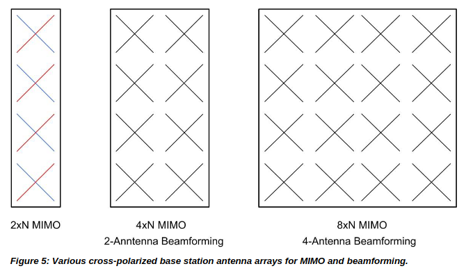
With this kind of antenna, single-codeword TM4 actually has an interpretation as “polarization-forming” (for lack of a better word). Rather than beamforming, the result of combining +45 and -45 deg polarizations with a phase offset that is an integer multiple of \(\pi/4\), is vertical, horizontal, RHCP, or LHCP polarization (depending on the choice of the precoding matrix). Therefore, we can think that if the eNB has CSI, it can choose the polarization among these 4 that best matches the receiver antenna polarization.
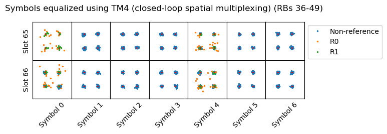
TM4 equalization in the recording
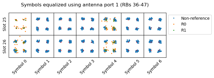
After all this theory, let us show the result of performing TM4 equalization for the PDSCH transmission corresponding to the DCI shown above. We can see that the constellation of the data symbols looks quite good.
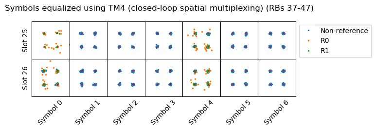
Recall that in this recording the channel amplitude response looks like this. In the higher frequencies of the cell (which is where this transmission takes place), port 1 is received much stronger than port 0. We can also see this in the equalized reference symbols R0 and R1 above. R0 is much noisier because it has less SNR.
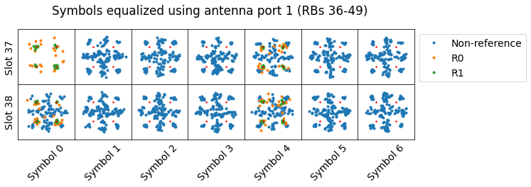
If we equalize this TM4 transmission as if it was a single-port transmission on port 1, we get the following constellation, which doesn’t look too bad. Indeed, the effect of doing this wrong equalization is to distort the constellation by a factor of \(h_0/h_1 + i\), which is close to a 90 degree rotation.
If we instead use transmit diversity equalization, the constellation is even worse, but still not too terrible. Intuitively speaking, this is because since in this case the channel response of one of the ports is much larger than the other, even though using the transmit diversity equalization formula is wrong in this case, the contribution of the terms that are multiplied by the smaller channel acts as a small inter-symbol interference (however, since in this case it is port 1 the port whose channel is largest, there are some complex conjugates, subcarrier swaps and sign inversions affecting the constellation, so even if it looks right, the bits decoded from it aren’t).

Another example of a single-codeword TM4 transmission in the recording is given by the following DCI, 0x7007ceeb0160, scrambled with C-RNTI 0xced8. Here the transmission uses two segments of resource blocks. The precoding matrix is the same as in the previous example.
The equalized symbols for the lower resource blocks and the upper resource blocks are shown here separately. Note that the two segments is somewhat different, since the channel response is quite different.
TM4 with two codewords
DCI and precoding matrix
In the recording that I used, there is one PDSCH transmission that uses TM4 with two codewords. This is its corresponding DCI in the PDCCH. We can see that the two codewords use the same MCS.
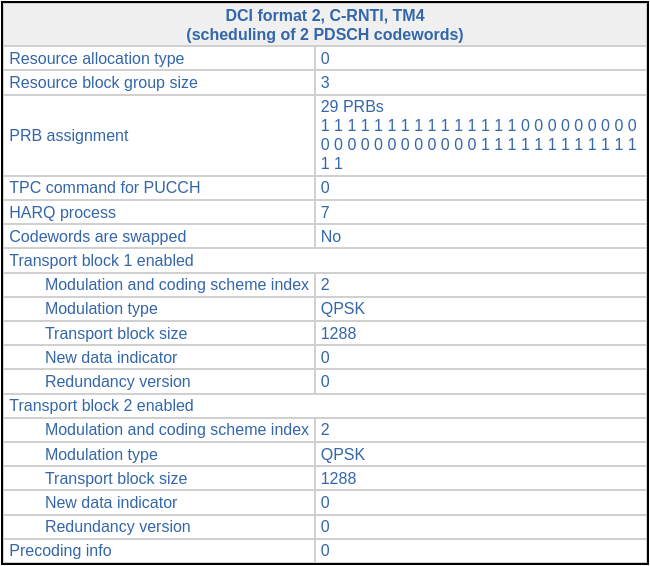
The precoding information field uses the same table as for one codeword. In this case, the value 0 indicates that the precoding matrix is\[\frac{1}{2}\begin{pmatrix} 1 & 1 \\ 1 & -1\end{pmatrix}.\]Note that as in the case of one codeword, the precoding matrices are normalized so that the sum of the power transmitted over the two antenna ports has an expected value of one if the symbols of each codeword are uncorrelated and have power one.
Equalization and SNR analysis for 2×2 MIMO
The following is a short treatment of 2×2 MIMO, as used in LTE TM4. The full theory of 2×2 MIMO is much more nuanced and admits many other techniques. We will be treating the cases of one codeword and two codewords at the same time and with the same notation, in order to compare them. We denote by \(x\) either a symbol from the single codeword, or a pair of symbols from each of the two codewords. Thus, \(x\) is either a complex scalar or a vector in \(\mathbb{C}^2\). We denote by \(W\) the precoding matrix, which is either 2×1 or 2×2. The vector of the symbols transmitted by each antenna port is\[y = Wx.\]We assume that the UE has two antennas, and denote by \(H\) the channel response between the two transmit and two receive antennas. This is a 2×2 matrix with entries \(h_{jk}\) that denote the channel between transmit port \(k\) and receive port \(j\). The UE receives the vector\[z = Hy + n = HWx + n.\]Here \(n\) denotes the receiver noise. We assume that its covariance is \(\mathbb{E}(nn^*) = I\). This can be assumed without loss of generality by multiplying \(z\) and \(H\) on the left by \(\mathbb{E}(nn^*)^{-1/2}\).
Assuming that \(W^*H^*HW\) is invertible, the UE can estimate \(x\) by computing\[\widehat{x} = (W^*H^*HW)^{-1}W^*H^*z = x + (W^*H^*HW)^{-1}W^*H^*n.\]We denote by\[\widehat{n} = (W^*H^*HW)^{-1}W^*H^*n\]the noise vector that affects the recovered symbols. Its covariance \(R\) can be computed as\[R = \mathbb{E}(\widehat{n}\widehat{n}^*) = (W^*H^*HW)^{-1}.\]It is now useful to consider the singular value decomposition of \(H\),\[H = U\Sigma V^*,\]where \(U\) and \(V\) are unitary and\[\Sigma = \begin{pmatrix} \sigma_0 & 0 \\ 0 & \sigma_1\end{pmatrix},\quad \sigma_0 \geq \sigma_1 > 0.\]Using this decomposition we have\[R = (W^*V\Sigma^2V^*W)^{-1}.\] Since\[\Sigma^2 = \sigma_1^2 I + (\sigma_0^2 – \sigma_1^2)e_0e_0^*,\]where \(e_0 = (1, 0)^T\), putting \(v_0 = Ve_0\) we get\[R = (\sigma_1^2 W^*W + (\sigma_0^2 – \sigma_1^2) W^* v_0 v_0^* W)^{-1}.\]
Now, in the single codeword case, \(W\) is a 2×1 vector which we denote by \(w\). The covariance \(R\) is the scalar\[R = (\sigma_1^2 \|w\|^2 + (\sigma_0^2 – \sigma_1^2) |\langle w, v_0\rangle|^2)^{-1}.\]We see that\[\|w\|^{-2}\sigma_0^{-2} \leq R \leq \sigma_1^{-2}\|w\|^{-2}.\]Moreover, if we have knowledge of the channel \(H\) and are free to choose \(w\) with a fixed \(\|w\|\), then we can obtain any value of \(R\) that satisfies the above inequalities by choosing \(w\) appropriately.
In the two codeword case, if we assume that \(W\) is unitary, then\[R = W^*V^*\Sigma^{-2}VW.\]We denote by \(r_j = e_j^* R e_j\) the covariance of the noise on each of the two recovered symbols. We have the condition\[r_0 + r_1 = \operatorname{tr}(R) = \operatorname{tr}(\Sigma^{-2}) = \sigma_0^{-2} + \sigma_1^{-2}.\]Moreover, \(r_j\) satisfy the inequalities\[\sigma_0^{-2} \leq r_j \leq \sigma_1^{-2}.\]If we have knowledge of the channel \(H\) and are free to choose the unitary \(W\), we can obtain any pair of values for \(r_0, r_1\) that satisfy these conditions. Indeed, putting \(v_1 = V^*e_1\), we have\[R = \sigma_0^{-2} I + (\sigma_1^{-2}-\sigma_0^{-2})W^*v_1v_1^*W,\]so\[r_j = \sigma_0^{-2} + (\sigma_1^{-2} – \sigma_0^{-2})|\langle W e_j, v_1\rangle|^2.\]
For a fair comparison between the one codeword case and the two codeword case, we assume that in the one codeword case \(\|w\| = \sqrt{2}\). This is so that the total transmitted power over the two ports is the same regardless of whether one or two codewords are transmitted. In fact, a look at the LTE precoding matrices table above shows that for two codewords all the precoding matrices are a 2×2 unitary times \(1/\sqrt{2}\), and for one codeword they all are a 2×1 vector with norm one.
There are different metrics with which the 1×1 and 2×2 covariances \(R\) can be compared. A usual choice is the channel capacity. For the one codeword case, the channel capacity is\[C = \log (1 + R^{-1})\]if we omit the constant factor that gives the bandwidth and the conversion from \(\log\) to \(\log_2\). We see that to maximize the capacity, it is necessary to make \(R\) as small as possible, which is quite intuitive. As seen above, the best we can achieve by choosing freely \(w\) with \(\|w\| = \sqrt{2}\) is \(R = \sigma_0^{-2}/2\). This corresponds to transmitting through the channel eigenmode that has maximum SNR. In this optimal case, the capacity is\[C = \log (1 + 2\sigma_0^2).\]
In the two codeword case, the capacity is the sum of the capacities for each codeword, so\[C = \log(1 + r_0^{-1}) + \log(1 + r_1^{-1}).\]Doing some algebra and using \(r_0 + r_1 = \sigma_0^{-2} + \sigma_1^{-2}\), we see that\[C = \log\left(1 + \frac{\sigma_0^{-2} + \sigma_1^{-2} + 1}{r_0r_1}\right).\]Hence, the maximum capacity is achieved by making the product \(r_0r_1\) as small as possible. Putting \(s = |\langle W e_0, v_1\rangle|^2\) and using \(|\langle W e_1, v_1\rangle|^2 = 1 – s\), we get\[r_0r_1 = \sigma_0^{-2}\sigma_1^{-2} + (\sigma_1^{-2} – \sigma_0^{-2})^2 s(1-s).\]Note that \(0 \leq s \leq 1\), and if we are free to choose a unitary \(W\), we can obtain any value of \(s\) satisfying this condition. The optimal capacity is achieved for \(s = 0\) or \(s = 1\). This choice corresponds to transmitting signals of equal power through the channel eigenmode that has maximum SNR (which corresponds to the singular value \(\sigma_0\)) and the eigenmode that has minimum SNR (which corresponds to the singular value \(\sigma_1\)). In this optimal case the capacity is\[C = \log\left(1 + \frac{\sigma_0^{-2} + \sigma_1^{-2} + 1}{\sigma_0^{-2}\sigma_1^{-2}}\right) = \log(1 + \sigma_0^2 + \sigma_1^2 + \sigma_0^2 \sigma_1^2).\]
Note that this optimal choice is not the same as the water filling algorithm. The water filling algorithm puts different power levels into each channel eigenmode, which cannot be done with a unitary precoding matrix \(W\). With the normalization we are doing, the water filling algorithm would give the solution \(q_0, q_1\) that maximizes\[C = \log((1 + q_0 \sigma_0^2)(1 + q_1 \sigma_1^2))\]subject to the conditions \(q_0 + q_1 = 2\) and \(q_j \geq 0\). The optimal solution for unitary precoding corresponds to the choice \(q_0 = q_1 = 1\), but in general there is a better choice of \(q_0, q_1\) that maximizes the capacity. This choice can be found using Lagrange multipliers. It is\[q_j = 1 + \frac{1}{2\sigma_0^2} + \frac{1}{2\sigma_1^2} – \frac{1}{\sigma_j^2}\]if this formula gives \(q_1 \geq 0\), or \(q_0 = 2\), \(q_1 = 0\) otherwise.
Let us now compare the capacities of the one codeword and two codeword cases when we can freely choose \(w\) with \(\|w\| = \sqrt{2}\) for the one codeword case and \(W\) a unitary for the two codeword case. We see that the two codeword case gives greater capacity whenever\[0 \leq \sigma_1^2 – \sigma_0^2 + \sigma_0^2 \sigma_1^2.\]This inequality holds whenever \(\sigma_1 \geq 1\), and also whenever\[\sigma_0^2 \leq \frac{\sigma_1^2}{1 – \sigma_1^2}.\]The intuition here is that the two codeword case gives better capacity unless the SNR of the weak eigenmode is low and the SNR of the strong eigenmode is large enough.
In LTE, however, the precoding matrix \(W\) cannot be chosen freely. There are only a few possible choices for it. For one codeword, with the normalization \(\|w\| = \sqrt{2}\), the possible choices are \(w = (1, i^k)^T\) for \(k = 0, 1, 2, 3\). Let us now study what is the best of these matrices to choose depending on the channel \(H\). The columns of the matrix \(V\) are eigenvectors of \(H^*H\). Since these eigenvectors are uniquely determined only up to multiplication by a complex scalar of modulus one, we can assume that \(V\) is of the form\[V = \begin{pmatrix}\cos \theta & – e^{-i\varphi}\sin\theta \\ e^{i\varphi}\sin\theta & \cos \theta\end{pmatrix}\]for \(\theta, \varphi \in \mathbb{R}\). These two parameters have the following geometric interpretation. If we consider a signal \(y\) transmitted by the two antenna ports of the eNB with total power one, \(\|y\|^2 = 1\), then the total power received at the two antenna ports of the UE is \(\|Hy\|^2\). The transmit vector \(y\) that maximizes \(\|Hy\|^2\) is in fact the first column of \(V\), this is, \(y = v_0 = V e_0\). This follows from \(\|Hv_0\|^2 = \|U\Sigma V^*V e_0\|^2 = \sigma_0^2\). Therefore, the parameter \(\theta\) indicates the power sharing between the two transmit ports in this particular maximal solution \(y = v_0\). A value of \(\theta\) close to something of the form \((2n+1)\pi/4\) gives near equal power sharing, while a value of \(\theta\) close to something of the form \(n\pi/2\) allocates all the power to one of the antennas. The parameter \(\varphi\) gives the phase offset that needs to be applied to the transmit ports in this solution \(y = v_0\).
I don’t know if there are assumptions that imply that in practical situations the value of \(\theta\) is more likely to be close to something of the form \((2n+1)\pi/4\) rather than to something of the form \(n \pi/2\). As we will see next, the precoding matrices in the LTE codebooks are not very good choices when \(|\sin 2\theta|\) is small.
Continuing with the one codeword case, by putting\[t = \frac{|\langle w, v_0\rangle|^2}{\|w\|^2},\]we have\[R = \|w\|^{-2}(\sigma_1^2 + (\sigma_0^2-\sigma_1^2)t)^{-1} = (2\sigma_1^2 + 2(\sigma_0^2-\sigma_1^2)t)^{-1}.\]Now we can compute\[t = \frac{1}{2}|\cos \theta + i^k e^{-i\varphi}\sin\theta|^2 = \frac{1 + \sin 2\theta \cos \left(\varphi – \frac{k\pi}{2}\right)}{2}.\]By an appropriate choice of \(k\) we can assume that\[\sin 2\theta \cos \left(\varphi – \frac{k\pi}{2}\right) \geq |\sin 2\theta| \frac{\sqrt{2}}{2},\]but since it can happen that \(\sin 2\theta = 0\), the only lower bound that we have for \(t\) that holds in all cases (choosing \(w\) appropriately depending on \(V\)) is \(t \geq 1/2\). This implies\[R \leq (\sigma_0^2 + \sigma_1^2)^{-1}.\]Therefore, the channel capacity satisfies\[C \geq \log (1 + \sigma_0^2 + \sigma_1^2).\]
For the two codeword case there are only two possible choices for the unitary precoding matrix \(W\):\[W = \frac{1}{\sqrt{2}}\begin{pmatrix} 1 & 1 \\ 1 & -1\end{pmatrix},\]and\[W = \frac{1}{\sqrt{2}}\begin{pmatrix} 1 & 1 \\ i & -i\end{pmatrix}.\]Observe that the four columns of these two matrices are the four vectors \(w\) that can be chosen for the one codeword case (scaled by a factor \(1/\sqrt{2}\)). Here we are concerned with computing the product \(s(1-s)\), where \(s = |\langle We_0, v_1|\rangle|^2\). The vector \(v_1\) is \(v_1 = (e^{i\varphi}\sin\theta, \cos\theta)^T\). For the first possible choice for \(W\) we have\[s = \frac{1}{2}|e^{i\varphi}\sin\theta + \cos\theta|^2 = \frac{1 + \sin 2\theta \cos \varphi}{2}.\]This gives\[s(1-s) = \frac{1-\sin^2 2\theta \cos^2 \varphi}{4}.\]A similar calculation shows that for the second possible choice for \(W\) we have\[s(1-s) = \frac{1 – \sin^2 2\theta \sin^2 \varphi}{4}.\]Selecting one of these two choices of \(W\) according as to whether \(\cos^2 \varphi\) or \(\sin^2\varphi\) is largest, we can achieve\[s(1-s) \leq \frac{1 – \frac{\sin^2 2\theta}{2}}{4}.\]However, as in the one codeword case, it can happen that \(\sin 2\theta = 0\), so the best upper bound that we can give for \(s(1-s)\) that holds in every case by choosing appropriately between the two precoding matrices \(W\) is\[s(1-s) \leq \frac{1}{4}.\]This bound is tight whenever \(\sin 2\theta = 0\). Such a bound also follows from the fact that \(0 \leq s \leq 1\), so this shows that when \(\sin 2\theta = 0\), the two precoding matrices that are available actually give the worst possible choices among all unitary matrices \(W\). The bound \(s (1 – s) \leq 1/4\) implies that the channel capacity satisfies\[C \geq \log\left(\frac{4(1+\sigma_0^2)(1+\sigma_1^2)\sigma_0^2\sigma_1^2}{4\sigma_0^2\sigma_1^2 + \sigma_0^2-\sigma_1^2}\right).\]
Here we have obtained lower bounds for the channel capacity in the one codeword and two codeword cases. These bounds are tight whenever \(\sin 2\theta = 0\). Unfortunately, comparing the two bounds to see which is greater does not give a simple expression in terms \(\sigma_0\) and \(\sigma_1\) (it involves solving a quadratic equation). We can compare the two bounds numerically. The following plot shows in black the region where the lower bound for two codewords is greater than the lower bound for one codeword. Since \(\sigma_0 \geq \sigma_1\), the upper-left triangle of the plot is not shaded in black.
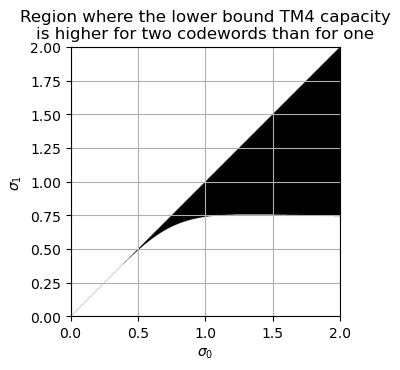
This plot shows that in practice, if \(\sigma_1 \geq 0.75\), then the two-codeword lower bound is higher, suggesting that in this condition two codewords will achieve higher capacity regardless of the geometry of the unitary \(V\).
Two-codeword TM4 and polarization diversity
As indicated above, a common antenna configuration for two-port eNBs is as cross-polarized antennas with +45 deg and -45 deg polarizations. Let us assume that the UE has two ports that are also in orthogonal polarizations. If the propagation path is polarization independent, then the matrix \(H\) is a positive constant \(\sigma\) times a unitary \(U\) that gives the transformation from the eNB polarization basis to the UE polarization basis. The singular value decomposition for \(H\) is \(H = U \Sigma V^*\) with \(\Sigma = \sigma I\), so that \(\sigma_0 = \sigma_1 = \sigma\), and \(V = I\). Applying the results of the previous section, we see that precoding with any vector \(w\) with \(\|w\| = \sqrt{2}\) in the one codeword case, and any unitary \(W\) in the two codeword case give optimal results regarding the channel capacity, because \(\sigma_0 = \sigma_1\).
In the two codeword case, the two available precoding matrices correspond to either transmitting one codeword in horizontal polarization and another codeword in vertical polarization, or to transmitting one codeword in RHCP and the other in LHCP. The UE can use the CRS (which have +45 deg and -45 deg polarizations) to estimate the polarization basis change that separates both codewords, namely \(H^{-1} = \sigma^{-1} U^*\). Therefore, two-codeword TM4 can be understood in this case as polarization diversity transmission.
In a more realistic situation, the propagation will depend somewhat on the polarization, so the matrix \(H\) will no longer be a multiple of a unitary. However, in good conditions it will still be close to a multiple of a unitary, and this reasoning will apply approximately, because \(\sigma_0/\sigma_1\) will be close to one.
Demodulation of two-codeword TM4 with a single antenna
As we have seen, two-codeword TM4 is intended to be received by a UE with two or more antenna ports. If a UE has only one antenna port, then the data received on each subcarrier gives only one equation for two unknowns (one symbol transmitted from each of the two codewords), so it cannot recover the transmitted data in general. It would seem that we cannot do anything to decode the two-codeword TM4 transmissions in the recording that I’m using in these posts, since the recording was done with a single antenna. However, with some ingenuity, I think that it is possible in some cases.
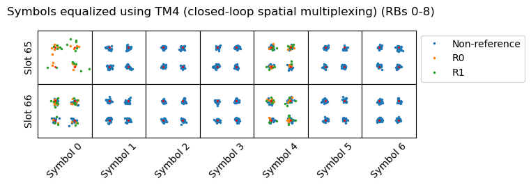
The following figure shows the upper resource blocks of the two-codeword TM4 transmission corresponding to the DCI shown above (recall that this transmission was split into two segments of resource blocks, one occupying the lower part of the cell and the other the higher part). Here it has been equalized using only the channel response for antenna port 1. The constellation we obtain looks quite curious. It is a cross and four QPSK points at amplitude \(\sqrt{2}\).
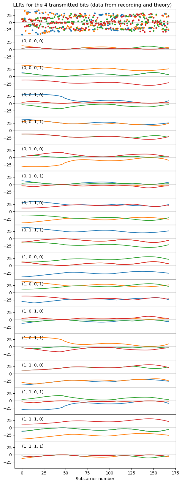
In order to understand better this constellation, it is good to simulate what happens if we take a two-codeword TM4 transmission, run it through the channel present in the recording, and equalize it with the channel for antenna port 1. Such a transmission carries 4 bits per subcarrier (2 bits for each of the QPSK constellations of each of the two codewords). Therefore, there are 16 different possible values that can be transmitted. We mark each of the 16 values with a different colour, and simulate what happens for each of the subcarriers in resource blocks 36-49, which are the ones occupied by the transmission we’re examining. The result corresponding to symbol 1 in slot 37 is shown here.
Comparing this with the data that we have demodulated from the recording , we see that it looks the same, plus noise.
To understand better why this constellation appears, first take into account that with the precoding matrix used in this transmission, port 0 is transmitting the sum of the symbols from the two codewords divided by \(\sqrt{2}\), and port 1 is transmitting the difference of the symbols divided by \(\sqrt{2}\) (the precoding matrix actually has a \(1/2\) factor rather than \(1/\sqrt{2}\), but as I have mentioned, in this recording the PDSCH transmissions are scaled with an additional \(\sqrt{2}\) compared to the CRS). Therefore, whenever the symbols in the two codewords are opposite, port 0 is transmitting a zero, and port 1 is transmitting a QPSK symbol with amplitude \(\sqrt{2}\). When we equalize with the CRS for port 1, we simply get this QPSK symbol with amplitude \(\sqrt{2}\).
When the symbols are not opposite, then port 1 can either transmit \(0\) if they’re equal, or one of \(\pm\sqrt{2}\) or \(\pm \sqrt{2}i\) if they have opposite real parts and equal imaginary parts or vice versa. Now we remember that the channel response for port 0 is smaller than the channel response for port 1, so whatever that port 0 transmits acts as a perturbation for the symbol transmitted by port 1, shifting the symbol somewhat in the constellation plot. For example, when port 1 is transmitting \(\sqrt{2}\), the possible two symbols that give this value are \((1 + i)/\sqrt{2}\) and \((-1 + i)/\sqrt{2}\), or \((1 – i)/\sqrt{2}\) and \((-1 – i)/\sqrt{2}\). In the first case, port 0 transmits \(\sqrt{2}i\), and in the second case port 0 transmits \(-\sqrt{2}i\). When received and equalized with the channel for port 1, the signal transmitted by port 0 will pull the constellation point in opposite directions for each of these options. The angle in which it’s pulled depends on the phase difference between the channels for port 1 and port 0. It turns out that for the upper frequencies of the cell, the phase difference is around -100 deg. So in this example the signal from port 0 pulls the symbol in a direction which is almost parallel to the real axis.
This is precisely what we see in the constellation above. The locations of the constellation symbols are dominated by what is transmitted by port 1, but the signal from port 0 splits apart the two symbol combinations that get mapped to the same signal in port 1, allowing us to distinguish them. The amplitude of the port 0 signal compared to the port 1 signal is large enough to make this splitting easy to detect, but small enough to make the constellation still look like something recognizable.
A way in which we can exploit this situation is, for each subcarrier, to interpret the received data equalized with port 1 as a weird 16-point constellation, and to compute log-likelihood ratios for each of the 4 bits transmitted by that subcarrier. To do this, I have made an educated guess of 0.15 for the noise standard deviation and computed the LLRs using the max*-safe function. In the plot below, the first panel shows the LLRs obtained from the recording data. The remaining plots show a simulation of how the LLRs would look like without any noise for each of the 16 possible combinations of 4 transmitted bits. We see that there are some bit combinations and areas of the spectrum that are particularly bad, with the LLR getting too close to zero, but in general the LLR is large enough that it is possible to decode the bit without errors despite the noise. Looking at the LLRs from the recording, there are some points clustered around the zero line, but most of them are well away from zero and can be decoded. Perhaps the Turbo decoder would be able to decode the two codewords with the LLRs obtained with this method.
Code and data
I have updated the LTE downlink Jupyter notebook with the calculations used in this post. The recording that I have used can be found here.
One comment