LTE downlink: synchronization signals

I have been posting about analysing LTE signals, with a focus on the structure of the pilot signals. I my two previous posts on this topic, I looked at the uplink using an IQ recording of my phone. Now I turn my attention to the downlink. I have done a short recording of the B20 band carrier of my local base station and I will be analysing it in this and future posts.

In this post, we will look at the primary synchronization signal (PSS) and secondary synchronization signal (SSS). These are the first signals in the downlink that a UE (phone) will attempt to detect and measure to estimate the carrier frequency offset, symbol time offset, start of the radio frames, cell identity, etc.

In an FDD system such as the one we are looking at here, the PSS is transmitted in the last symbol of slots 0 and 10 in each radio frame (Recall that LTE FDD signals are organized in 0.5 ms slots each containing 7 OFDM symbols. A radio frame lasts 10 ms and contains 20 slots). The SSS is transmitted on the symbol before the PSS.

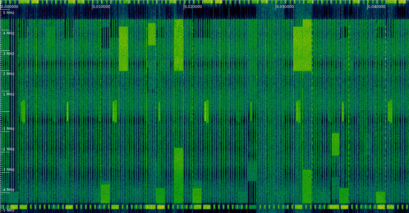
The figure below shows the waterfall of the first 20 ms of the recording. I have marked the locations of the PSS and SSS with a red tick. These signals only occupy the 6 central resource blocks (1.08 MHz), so that they are compatible with all the possible cell bandwidths (LTE supports cell bandwidths of 1.4, 3, 5, 10, 15 and 20 MHz) and can be received by a UE which doesn’t know the cell bandwidth yet. In this case, we are looking at a 10 MHz cell, and we can see the neighbouring 10 MHz cells in the top and bottom of the waterfall.

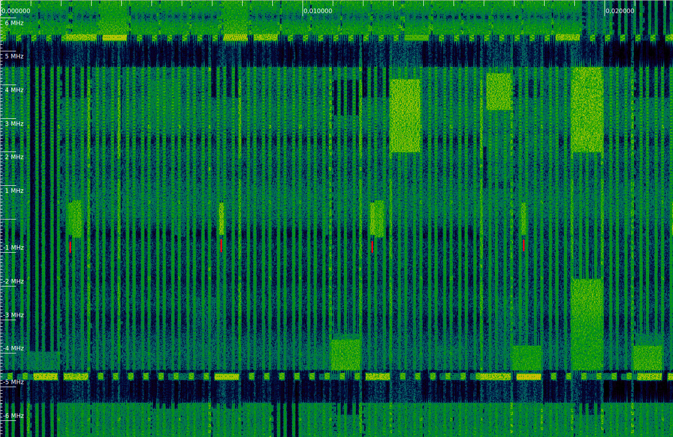
We can see that every other PSS and SSS transmission there is another 1.08 MHz transmission following it. This corresponds to the PBCH (physical broadcast channel), which is transmitted on the first 4 symbols of slot 1 in each radio frame. The keen reader will have noticed that the PBCH is slightly wider than the PSS and SSS. This is because the PSS and SSS only use the central 62 out of 72 subcarriers in the 6 resource blocks they occupy, leaving 5 subcarriers at each edge as a guardband. This helps UEs having a large carrier frequency offset to detect these signals. On the other hand, the PBCH occupies all the 72 subcarriers.

Recording set up

For this recording, I wanted to record the base station whose signal I receive at home. This has the fun part of driving around town to discover where my LTE coverage actually comes from. It could also become handy in case I want to do more recordings at home and know that it’s the same cell and how it is set up. In order to simplify the first analysis, I wanted a strong line-of-sight signal, which justifies the need of finding the cell site and travelling close to it.

This cell uses Vodafone’s 10 MHz carrier at 806 MHz in the B20 band (here you can see how in Spain Orange, Vodafone and Movistar have each a 10 MHz allocation at 796 MHz, 806 MHz and 816 MHz respectively, thus occupying the whole 30 MHz-wide B20 band). The PCI (physical cell ID) of the cell I want is 378.

With the help of Gqrx to monitor the spectrum (using a USRP B205mini and the 145/435 MHz vertical antenna on my car, which is not ideal but works), and LTE discovery to check the PCI of the cell that my phone was connected to, I drove around town and found the cell site. Interestingly, it is located at Movistar Plus+‘s headquarters.

I think that in this site there are collocated cells for Orange, Vodafone and Movistar. Since I was recording at 30.72 Msps, we can see the full B20 band. The 10 MHz carriers of the three companies are equally strong (and indeed quite strong, since I was ~100 metres away from the antennas and with line-of-sight).

While driving around, I observed that my phone preferred to use the B3 band cells at 1835.10 MHz (these are 20 MHz cells). Luckily, the B20 and B3 cells seem to be collocated and use the same PCIs, so I could deduce what was present on the B20 band by looking at what my phone was doing on B3.

I think that this cell site has antennas at 3 different corners of the Movistar Plus+ building (not all of the antennas are well visible from street level, and the Google maps satellite view is not too clear). They are used to beam in three different directions using three PCIs in the same group (meaning they use the same \(N_{ID}^{(1)}\) and different \(N_{ID}^{(2)}\)’s). I think this is a relatively common approach, but don’t quote me on that, since I haven’t found much documentation to this respect. For Vodafone, PCI 378 beams south-west (this is the cell I receive at home), PCI 379 beams north, and PCI 380 beams south-east. Unfortunately, I didn’t find a good way to have a clear line-of-sight to the PCI 378 antennas from street level, so I ended up recording the PCI 380 antennas.

To record, I used a PCB Vivaldi antenna (this was a gift from SkySafe to the attendees of GRCon 19) and the USRP B205mini, with only a short SMA cable (RG316, I think) between them. I held the antenna in vertical polarization (later I learned that LTE signals are often transmitted at +45º and -45º linear polarizations, so maybe this is not the best choice for recording).

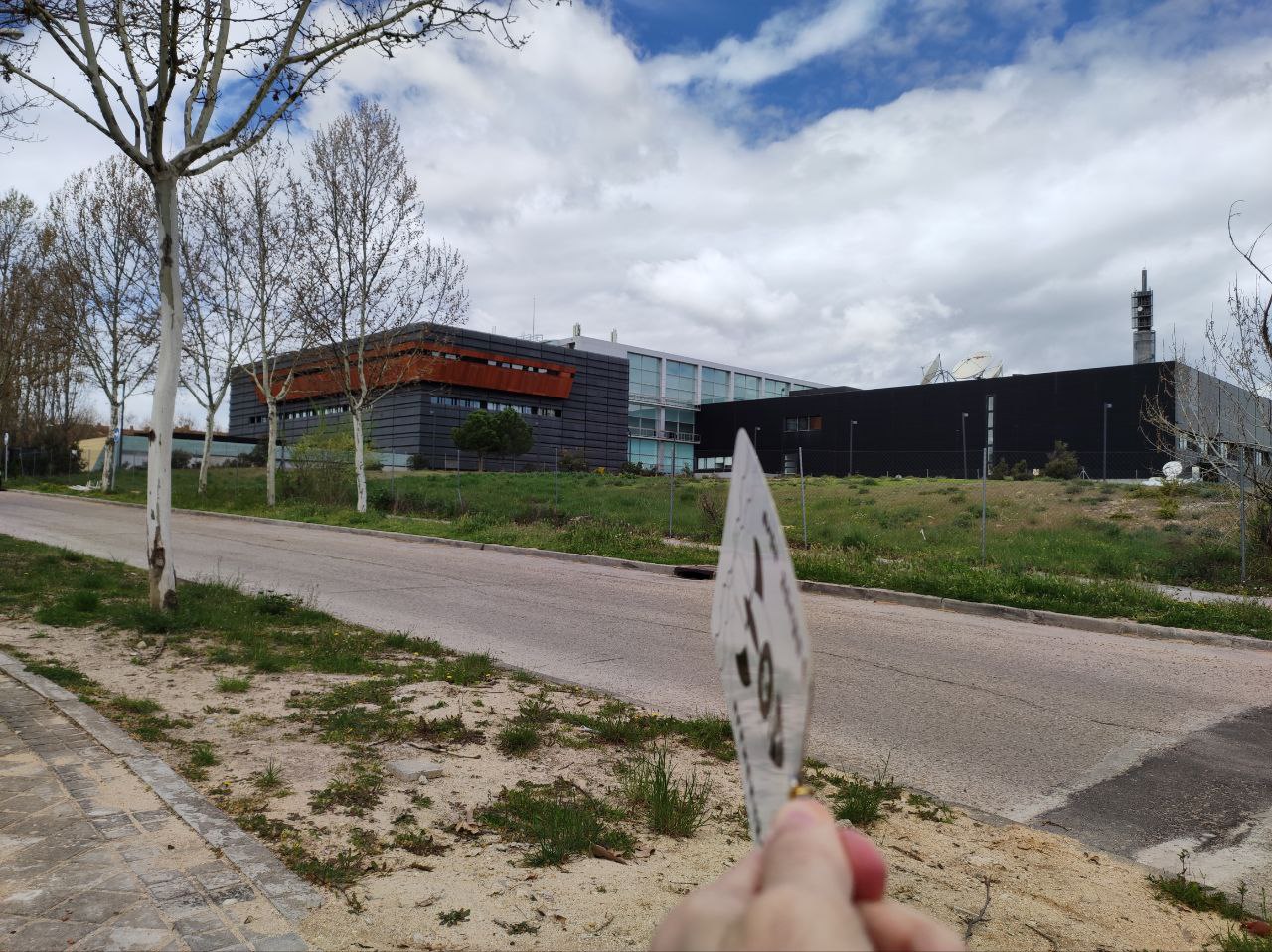
The photo below shows the location from which I recorded (see the corresponding Google street view). The LTE antennas are on the corner of the rooftop of the white building.

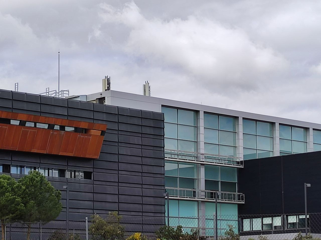
The next photo shows a zoomed-in view of the antennas on the rooftop.

The recording is 37 seconds long, essentially limited by how much I could record to RAM in my laptop. Here we will only be using the first second. I have shared this one second excerpt as the SigMF recording LTE_downlink_806MHz_2022-04-09_30720ksps SigMF here.

Primary Synchronization Signal structure

The LTE downlink signal does not use the DC OFDM subcarrier, in order to avoid problems in the transmitters and receivers related to local oscillator leakage, ADC response, etc. The PSS and SSS occupy 62 subcarriers symmetrically: 31 below DC, and 31 above DC. Additionally, 5 extra subcarriers at the edges are left as guard bands (and nothing is transmitted in these subcarriers during PSS and SSS transmissions).

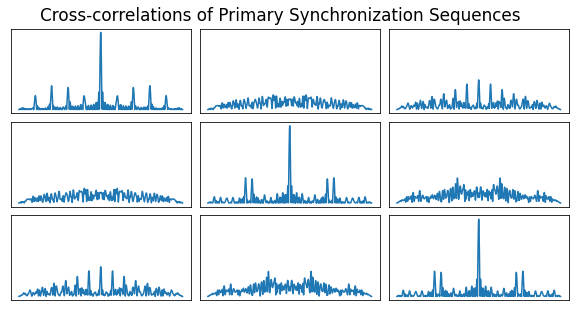
The OFDM symbol for the PSS is constructed using a Zadoff-Chu sequence of length 63\[x(n) = e^{-i\pi u n (n+1)/63},\quad n = 0, 1, \ldots, 62.\]The term \(n=31\) in this sequence is not used, since it would correspond to the DC subcarrier, and the remaining terms are mapped to the 62 PSS subcarriers. Zadoff-Chu sequences typically have good properties, such as constant modulus in the time and frequency domains, and low cross-correlation for sequences using different \(u\) parameters. However, only the sequences of prime length have all these good properties. Here we are using length \(63 = 3^2 \cdot 7\), which isn’t prime by any means. Moreover, we are zeroing out one of the terms in the sequence. This means that we lose these properties to some extent.

There are three different PSS that can be used, which correspond to the choices \(u = 25, 29, 34\). The value of \(u\) is chosen in terms of the cell number \(N_{ID}^{(2)}\), which is an integer between 0 and 2 that is related to the PCI via the formula\[PCI = 3N_{ID}^{(1)} + N_{ID}^{(2)}\](here \(N_{ID}^{(1)}\) is the cell group number and is an integer between 0 and 167).

The figure below shows the time-domain cross-correlations of the three PSS choices. Each choice corresponds to a column or row, so the diagonal shows the autocorrelations. We see that the sequences for \(N_{ID}^{(2)} = 0\) and \(N_{ID}^{(2)} = 2\) have a relatively large cross-correlation at a lag of zero. This is not very convenient, because it means that these signals will interfere with each other to some extent. For instance, if one of the two signals is present with large amplitude and we want to find whether the other signal is present with smaller amplitude, the cross-correlation is going to make this more tricky.

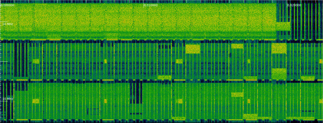
As we have seen in previous posts, Zadoff-Chu sequences are chirp-like, and so with the appropriate time-frequency resolution their waterfall can look like a set of diagonal bands. This makes it possible to distinguish the SSS and PSS symbols in the waterfall. The figure below shows the SSS and PSS transmission, followed by the PBCH. Note the different “texture” of the SSS and PSS symbols. Markers delimiting the symbols of the first two slots of the frame are included for clarity.

Detection of the Primary Synchronization Signal

All the signal processing and the plots in this post have been done in this Jupyter notebook.

The signals in the recording correspond to PCI 378, 379 and 380. All these have \(N_{ID}^{(1)} = 126\), and their \(N_{ID}^{(2)}\) is equal to 0, 1, and 2 respectively. Therefore, in what follows we will use the terms PCI 378, 379 and 380 and \(N_{ID}^{(2)} = 0, 1, 2\) somewhat interchangeable to refer to the three cells in this site.

To detect the PSS, I have generated time-domain versions of the OFDM symbols corresponding to each of the 3 possible PSS choices, and then correlate the first 5 ms of the recording against these. Since the carrier frequency offset is not too large, it is not necessary to search at multiple carrier frequencies. Later on, the carrier frequency offset is measured using the phase rotation between the SSS and PSS, and we see that it is approximately -1300 Hz.

The figure below shows the results of this correlation. We see a very clear peak corresponding to \(N_{ID}^{(2)}=2\). This is to be expected, since it is the cell number that corresponds to PCI 380. There is also a weaker peak for \(N_{ID}^{(2)}=0\), but this is caused by the cross-correlation we have shown above. As we will see later, the signals for PCI 378 and PCI 379 are also present in this recording, but they are 20 to 30 dB weaker than the signal for PCI 380, so it is a bit tricky to detect them.

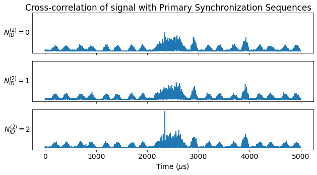
The next figure shows a zoom-in to the location where the peak appears. The peaks for \(N_{ID}^{(2)}=0\) and \(N_{ID}^{(2)}=2\) appear exactly at the same moment in time.

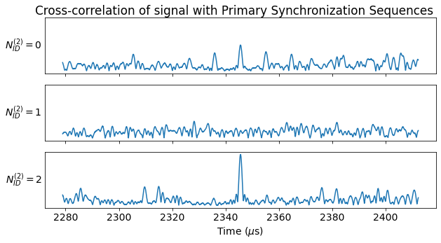
From the location of the correlation peak we obtain the time at which the PSS symbol starts. Since the PSS is about 1 MHz wide, the correlation peak has a width of around 1 microsecond, and given that the SNR is very good, the location of the peak can be detected quite accurately, so this gives us quite good synchronization (on the order of 10s of nanoseconds, as we will see).

PSS symbol analysis and equalization

Once that we have the symbol time offset obtained from the correlation with the PSS, we can demodulate the PSS OFDM symbols by performing an inverse Fourier transform. We will only look at the first second of the recording.

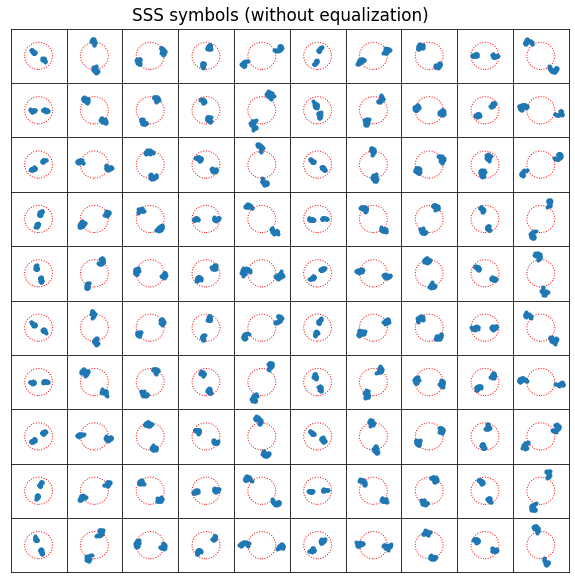
The figure below shows the first 100 PSS symbols as a 10×10 grid that should be read from left to right and top to bottom. The unit circle is shown for reference.

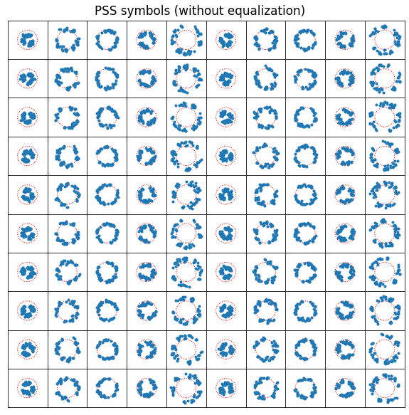
We note that the amplitudes of the PSS symbols follow a pattern that repeats every 5 half-frames. In fact, this behaviour can also be seen in the waterfall. It is noticeable that the 1st and 6th PSS transmissions are the weakest, while the 5th is the strongest.

I think that this is caused by transmit beamforming. There are five different beams that can be used to transmit the PSS and SSS, and they are used in sequence. This makes sense, because a UE that receives the cell with less SNR will have a better chance to receive the synchronization signals one out of five transmissions, when it happens to be in the beam that is used. I don’t know most of the details of how beamforming is used in LTE, so I could be saying something wrong here.

Since we know the Zadoff-Chu sequence for \(N_{ID}^{(2)}=2\) used to construct the PSS, we can wipe the sequence off, obtaining the following.

This now can be used to measure the channel response and perform equalization. We consider a very simple channel response model which has a single time-domain tap. To estimate the channel, we compute the average amplitude and fit a degree 1 polynomial to the phase versus frequency.

The figure below shows the amplitude and group delay of the estimated channel. The PSS transmissions have been classified in groups of 5 according to their half-frame number modulo 5. This makes clear the differences in power in what I believe to be different beams. The difference between the strongest and weakest beam is 8.6 dB.

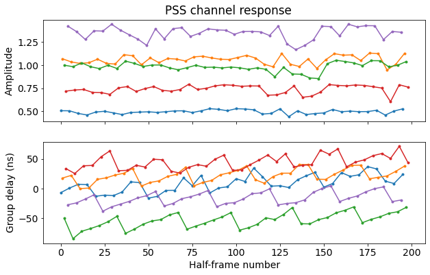
We also use the group delay estimate to correct the sampling frequency offset. In the plot above, a sampling frequency offset of 1.5 ppm has already been corrected. What we do to compute the start of each PSS symbol is to use the time estimate we obtained for the first one, compute a nominal time difference of 5 ms between PSS symbols and apply the 1.5 ppm correction to that, and round the result to the nearest sample (at 30.72 Msps). This rounding causes the staircase pattern in the group delay estimate. We see that despite the 1.5 ppm correction, the group delay keeps growing slowly, so the correction is not perfect.

Each of the five beams shows different group delays, with differences as large as 80 ns. I think that the group delay difference could be caused by the electronics of the beamformer. It doesn’t seem likely that this is a physical delay caused by different free space propagation paths, since 80 ns is equivalent to 24 metres. Another possible explanation is that the beamforming is done by two separate antennas a few tens of metres apart (in fact two groups of antennas can be seen in the photos, and having antennas separated several wavelengths is important for spatial diversity). Then, depending on how beamforming is done, the apparent group delay centre could move between the two antennas.

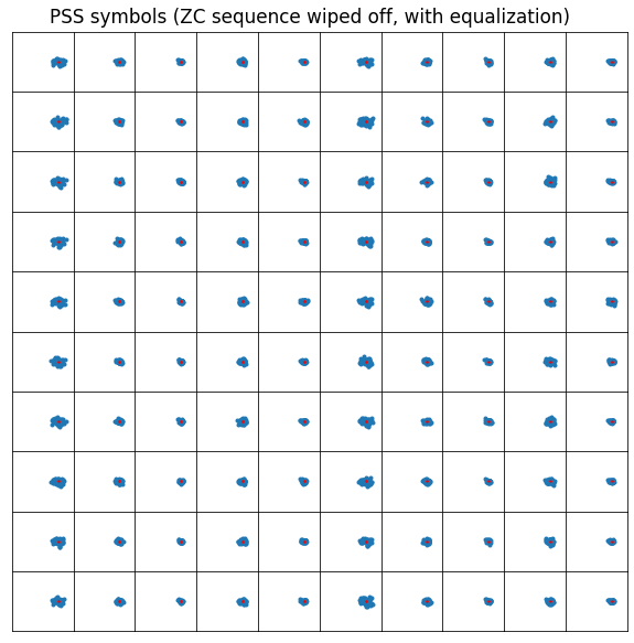
After equalization, we obtain the following PSS symbols, where the nominal constellation point (which is the complex number 1) has been marked with a red dot as a reference.

Detection of the PSS for PCIs 378 and 379

As we have remarked, the signal from PCI 380 is very strong in this recording, since we have the antennas in line-of-sight and we are inside the beam of this cell. Nevertheless, the signals from the other cells at this site, PCI 378 and 379 are also present in the recording.

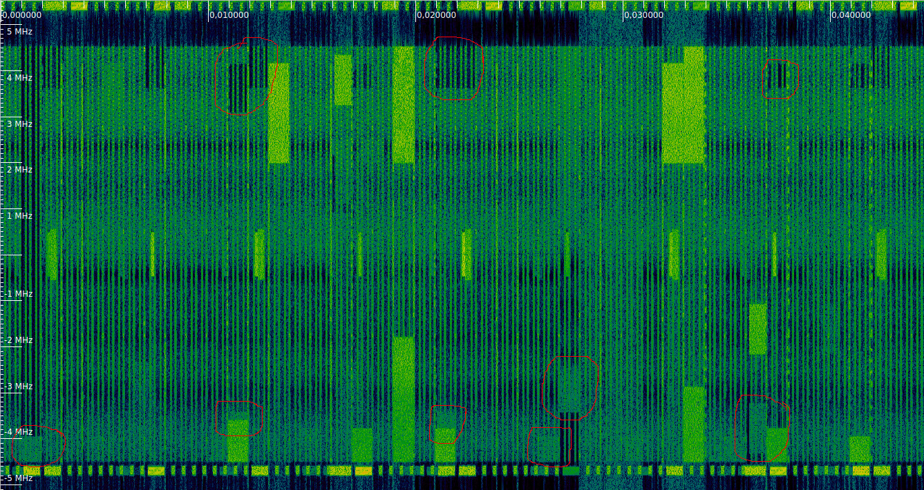
Indeed, we can even see the different cells by carefully looking at the waterfall. The much stronger transmissions correspond to PCI 380. But we also see some weaker transmissions “in the background” that correspond to other cells. In the figure below, almost all the time the full bandwidth of the cell is used by one of these background cells. However, we can also spot a few unused time-frequency regions. This cell has a certain peculiar amplitude versus frequency response, due to its channel. By looking at changes in the amplitude response, we can spot some transmissions of another cell of similar strength that has a different channel. I have marked some of these, as well as unused gaps in red.

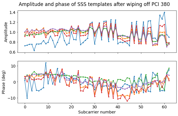
To study the PSS for the weaker cells PCI 378 and 379, first we form PSS “templates” by averaging all the PSS symbols (after wipe-off and equalization) in each of the five groups we have made corresponding to the transmit beams. This is reasonable, as it helps increase the SNR, and the PSS symbols in each group are similar, so we don’t destroy information by averaging.

The figure below shows the amplitude and phase of the resulting PSS templates. We can see two things. First, the overall amplitude and phase response is not flat, but has some curvature. Second, there is a pattern superimposed on the PSS symbols. This is specially noticeable in the amplitude. This pattern is caused by the PCI 378 and PCI 379 signals.

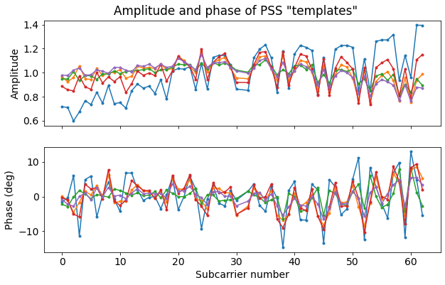
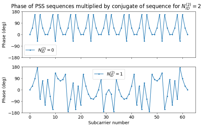
To understand this pattern in more detail, it helps to plot the phase of the sequence that is obtained by multiplying the PSS sequences corresponding to \(N_{ID}^{(2)} = 0, 1\) by the conjugate of the sequence corresponding to \(N_{ID}^{(2)}=2\), which is what we have used for wipe-off. What we obtain for \(N_{ID}^{(2)} = 0\) has a very characteristic pattern with a period of 7 subcarriers. We can see this kind of pattern in the right-hand side of the amplitude plot above.

The pattern for \(N_{ID}^{(2)} = 1\) has more variation, but we can recognise some of the “fast changes” in the left-hand side of the amplitude plot above.

In summary, what happens in this recording is quite peculiar and interesting. The PCI 378 signal is stronger than the PCI 379 signal. Therefore, the pattern we see in the PSS templates is dominated by the pattern for \(N_{ID}^{(2)} = 0\). However, the amplitude response of the channel for PCI 378 has a certain variation with frequency, and in fact the signal of this cell is weaker in the left-hand side of the PSS. In these subcarriers, the signal for PCI 379 dominates, and its corresponding pattern emerges.

As an additional remark, the previous plot shows why perhaps the three PSS sequences that 3GPP has chosen do not behave so well regarding the cross-correlation. The product of the sequence for \(N_{ID}^{(2)} = 0\) and the complex conjugate of the sequence for \(N_{ID}^{(2)} = 2\) doesn’t look any random. This is because the difference of the \(u\) parameters used by these sequences is 9 (it is 34 – 25). This divides 63, and the quotient is 7. The consequence is that the product then is equal to a Zadoff-Chu sequence of length 7, extended periodically to the 63 subcarriers.

It would have been beneficial to choose the three parameters \(u_1, u_2, u_3\) such that not only each \(u_j\) is coprime with 63, but also so that the differences \(u_j – u_k\), for \(j \neq k\), are coprime with 63. Unfortunately, there is no such choice. Moreover, it is neither possible to choose the \(u_j\) such that they are all coprime with 63, two of the pairwise differences are coprime with 63, and the other one is 7 (which would give a sequence of period 9 instead of period 7). Thus it seems that we are stuck with having a sequence of period 7 as the least bad thing we can do.

I wonder why 3GPP chose to use Zadoff-Chu sequences of length 63 for the PSS rather than length 61, which is prime. This might have given better cross-correlation properties.

The first step in trying to measure the PSS for PCI 378 and 379 is to equalize the channel for PCI 380 better so as to remove its contribution in the best possible way. However, the presence of the weaker signals from PCI 378 and 379 gets in the way, specially because of the large correlation between the PSS sequences for PCI 378 and 380. We will do an iterative approach.

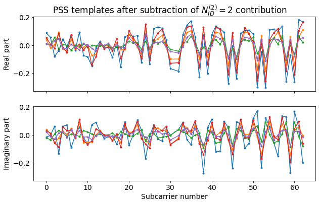
We start by fitting polynomials of degree 4 to the amplitude and phase of each of the PSS templates. The polynomials are shown below as a dashed line.

We use these polynomials to synthesize the contribution of the \(N_{ID}^{(2)} = 2\) PSS and subtract it from the templates. We obtain the signals shown below. It is clear that the pattern caused by \(N_{ID}^{(2)} = 0\) is much stronger in the higher subcarriers.

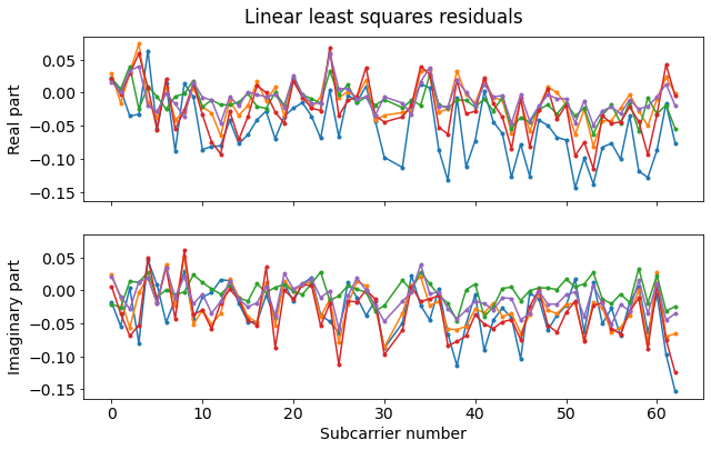
To take into account the effects of an amplitude versus frequency slope in the channel response for PCI 378 and PCI 379, we consider independent variables \(\delta_1\) and \(\delta_2\) that indicate these slopes. For each of the points in a grid covering the range \(|\delta_j| \leq 0.2\) 1/subcarrier, we perform a linear least squares fit to the data shown in the previous plot using the patterns for \(N_{ID}^{(2)} = 0\) and \(N_{ID}^{(2)} = 1\) with the slopes \(\delta_1\) and \(\delta_2\) applied. Then we look at the residuals of all these least squares to choose the best values for \(\delta_j\).

The figure below shows the least squares residuals depending on \(\delta_1\) (vertical axis) and \(\delta_2\) (horizontal axis) for each of the five templates. We see that there is an area of \(\delta_1\) that makes the residual decrease noticeably, while the value of \(\delta_2\) does not have much impact on the residual.

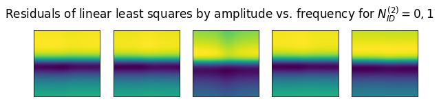
For this reason, we choose as \(\delta_1\) the values where the minimum is attained (giving values between 0.022 and 0.046 in units of 1/subcarrier), and fix \(\delta_2 = 0\).

Now we perform again a linear least squares with these fixed values of \(\delta_1\) and \(\delta_2\). The residuals are shown below. We can see that the real part is not quite flat. It has some undulation. This is caused by errors in the equalization of PCI 380.

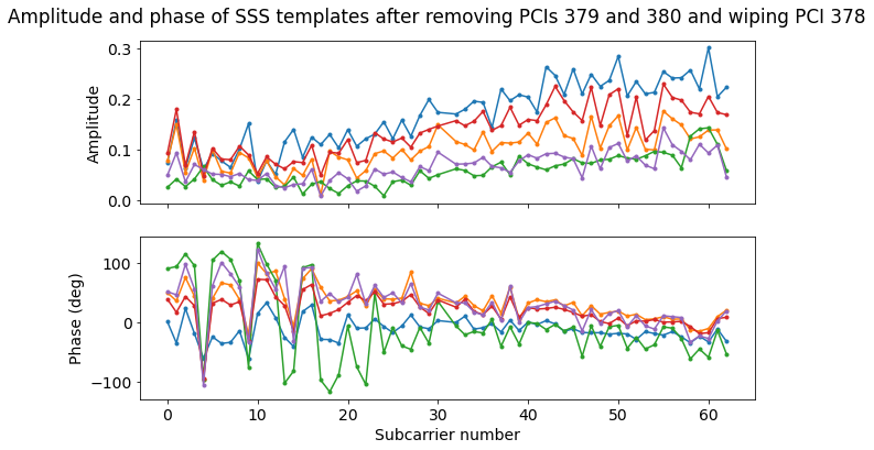
Now we improve our equalization of PCI 380. We use the least squares solutions for PCI 378 and 379 to subtract their contributions from the original PSS templates. The result is shown in the figure below. We see that the pattern for PCI 378 has almost disappeared, while there still remain some traces of a pattern that we may attribute to PCI 379.

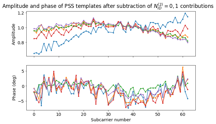
We can now perform again the polynomial fit using this data (also with polynomials of degree 4). The plot below shows the results. The new polynomial fit is shown as a dashed line, while the previous fit is shown as a dotted line. We can see that, specially in the blue curve, the old amplitude fit had larger values (and was a worse fit) than the new fit. This is caused by the cross-correlation of the \(N_{ID}^{(2)} = 0\) and \(N_{ID}^{(2)}= 2\) PSS. If we look at the effects caused by the pattern for \(N_{ID}^{(2)} = 0\) in the amplitude in the figures above, we see that most of the subcarriers have a positive going effect, which biases the first fit.

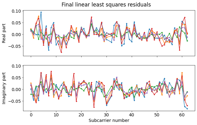
Using this new channel response for PCI 380 and the previously obtained values of \(\delta_1\) and \(\delta_2\) for PCI 378 and 379, we perform a linear least squares fit to the data using the sequences for PCI 378, 379 and 380. As expected, the coefficients we obtain for the PCI 380 sequence are very close to one. The residuals are shown here.

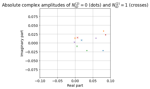
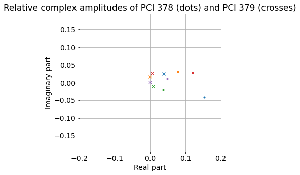
We can plot the coefficients corresponding to PCI 378 and PCI 379 for each of the templates. These give the amplitude and phase of the PCI 378 and 379 signals for each beam relative to the amplitude and phase of PCI 380 for that beam.

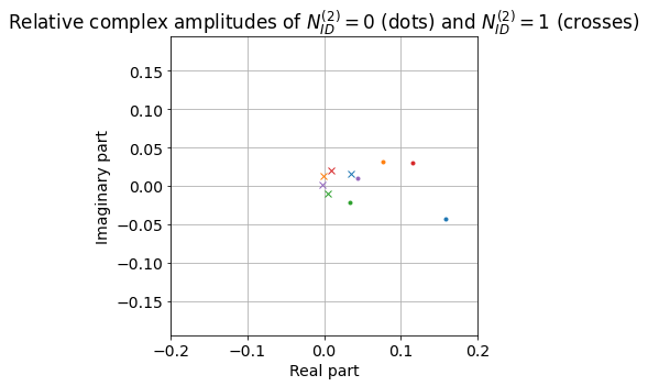
It is quite interesting too see the range over which the phases vary, specially for PCI 378. The first remark is that, for each beam the phase remains consistent in each PSS transmission (this cannot really be seen in this plot, since we have started by averaging over several transmission to form the templates, but we will see this effect below). This means that the transmitter carrier phases are synchronized.

Second, the phases for PCI 378 are spread over a region of only ~60 degrees, rather than over all the unit circle. It isn’t easy to interpret what this means, because we don’t know anything about the instrumental effects caused by the electronics in the phases of each of the beams.

Finally, it is interesting that the phases are located following what seems to be a circumference arc. This behaviour also happens for PCI 379 and in fact the phases appear in the same order there.

In the plot above we are using the power of each beam for PCI 380 as a reference. Since we have seen that each of these beams has a different power, it probably makes more sense to use an absolute scale for the power. In this way, we can represent the power of each beam of PCI 378 and 379 independently of what happens with PCI 380. Note that we can only do this for the amplitude. As we do not have a way to get an absolute phase reference, we still use the phase of PCI 380 as a reference. This absolute scaling is shown below.

Structure of the Secondary Synchronization Signal

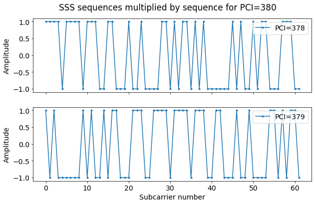
The 62 subcarriers of the SSS are modulated in BPSK, using the constellation points 1 (to encode the bit 0) and -1 (to encode the bit 1). The sequence is formed by interleaving two 31 bit sequences. If we denote the sequence of 62 subcarriers by \(d(n)\), \(n = 0, 1, \ldots, 61\), then the sequences \(d(2n)\) and \(d(2n+1)\), \(n = 0, 1, \ldots, 30\), are constructed separately. M-sequences are used as the basic construction block of these two 31-bit binary sequences. There are three different M-sequences, which are called \(s(n)\), \(c(n)\) and \(z(n)\). Their definition can be found in 3GPP TS 36.211.

Circular shifts of these sequences depending on the PCI are used. From the \(c(n)\) sequence, two sequences \(c_0(n)\) and \(c_1(n)\) are constructed using the value of \(N_{ID}^{(2)}\) as\[\begin{split}c_0(n) &= c((n+ N_{ID}^{(2)}) \mod 31),\\c_1(n) &= c((n + N_{ID}^{(2)} + 3) \mod 31).\end{split}\]

A pair of integers \(m_0\) and \(m_1\) between 0 and 30 are computed from the value of \(N_{ID}^{(1)}\) using some relations that appear in TS 36.211. These as used to define\[\begin{split}s_0(n) &= s((n+m_0) \mod 31),\\ s_1(n) &= s((n+m_1) \mod 31),\end{split}\]as well as\[\begin{split}z_0(n) &= z((n+(m_0 \mod 8)) \mod 31),\\ z_1(n) &= z((n+(m_1 \mod 8)) \mod 31).\end{split}\]

In the case of the PSS, the same sequence is transmitted in each half-frame (i.e., every 5 ms). Therefore, a UE that detects the PSS only achieves time synchronization modulo 5 ms. In order to give synchronization to the 10 ms frame, two different sequences for the SSS are used alternatively. In the first slot of a frame (i.e., in the first half-frame), the SSS is defined by\[\begin{split}d(2n) &= s_0(n) c_0(n),\\ d(2n+1) &= s_1(n) c_1(n) z_0(n).\end{split}\]In the eleventh slot of a frame (i.e., in the second half-frame), the SSS is defined by\[\begin{split}d(2n) &= s_1(n) c_0(n),\\ d(2n+1) &= s_0(n) c_1(n) z_1(n).\end{split}\]Note that if we take the rule that the sequence \(z_j(n)\) that is used for the odd terms \(d(2n+1)\) has the same index \(j\) as the sequence \(s_j(n)\) used for the even terms \(d(2n)\), then the only change between the first and eleventh slots consists in swapping \(s_0(n)\) and \(s_1(n)\). In fact, \(c_0(n)\) is always used for the even terms and \(c_1(n)\) is always used for the odd terms. This property will be important when we try to find the \(N_{ID}^{(1)}\) and whether the slot is the first or tenth, starting from some particular SSS.

Also, note that the sequences \(c_j(n)\) only depend on the cell number \(N_{ID}^{(2)}\) and the sequences \(s_j(n)\) and \(z_j(n)\) only depend on the cell group number \(N_{ID}^{(1)}\). We will use this property when we try to separate the signals corresponding to PCI 378, 379 and 380, which all have the same \(N_{ID}^{(1)}\).

Detection of the SSS and calculation of the PCI

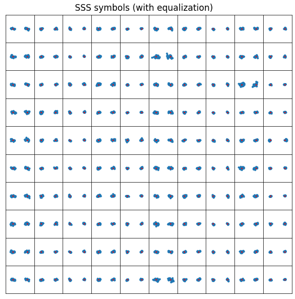
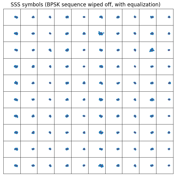
We can demodulate the OFDM symbols of the SSS in the same way as we have done with the PSS. The image below shows the first 100 SSS transmissions as a 10×10 grid. We can already see the BPSK constellation. The unit circle is shown in red as a reference.

Applying the equalization we have computed for the PSS (including the final equalization with degree 4 polynomials) we obtain the following. The constellations points 1 and -1 are shown as red dots for reference.

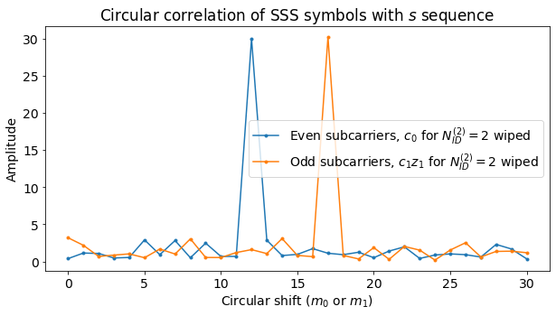
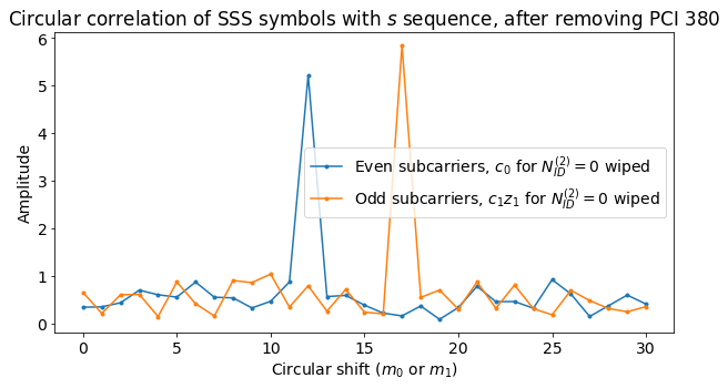
Now we take the first SSS transmission and use it to find the value of \(N_{ID}^{(1)}\) (which we already know should be 126, but we will use this as a cross-check). To do this, first we can compute \(c_0(n)\) and \(c_1(n)\), as they only depend on \(N_{ID}^{(2)}\), which we have already found with the PSS. We denote by \(d(n)\) the SSS sequence that we have received. We form the product \(d(2n) c_0(n)\) and compute its circular correlation with \(s(n)\). This will have a peak at the position \(m_j\), where \(j = 0\) if the SSS corresponds to the first half-frame and \(j = 1\) otherwise.

Then we use this value of \(m_j\) to compute \(z_j(n)\). Now we can form \(d(2n+1) c_1(n) z_j(n)\). We compute the circular correlation of this product with \(s(n)\). The peak position is \(m_{1-j}\). Now that we have the values of \(a=m_j\) and \(b=m_{1-j}\) (but we don’t know yet if \(j = 0\) or \(j=1\)), we can use the table of pairs \((m_0, m_1)\) versus \(N_{ID}^{(1)}\) and search if any of the pairs \((a,b)\) or \((b,a)\) appears there. If we find one of these pairs, this gives whether \(j = 0\) or \(j = 1\) and the value of \(N_{ID}^{(1)}\) (the table has the property that if a tuple \((a,b)\) appears in the table, then \((b,a)\) does not appear).

The figure below shows the two circular correlations. Their peaks give the pair \((a, b) = (12, 17)\), from which \(j = 0\) and \(N_{ID}^{(1)} = 126\) is found.

Now that know the \(N_{ID}^{(1)}\) and \(N_{ID}^{(2)}\), we can generate the SSS symbol sequences for each half-frame and use them to wipe the received SSS symbols. We obtain the following constellations, where the point 1 is marked in red as a reference.

Detection of the SSS for PCIs 378 and 379

In order to detect the SSS for the weaker cells PCI 378 and 379, first we form SSS “templates” with the received data as we did with the PSS. To construct these templates we use the data after equalization and wipe-off of PCI 380. Having wiped off PCI 380 allows us to average the SSS transmissions in the first half-frames and second half-frames together, as the wipe off eliminates all the differences that the SSS presents depending on which half of the frame it is transmitted.

In fact, as we have remarked above, the sequences \(s_j(n)\) and \(z_j(n)\) only depend on \(N_{ID}^{(1)}\). Therefore, the wipe-off for PCI 380 also wipes these sequences in the contribution of PCI 378 and 379 to the received SSS. The terms that remain in these contributions are products of \(c_j(n)\) for \(N_{ID}^{(2)} = 0, 1\) and \(c_j(n)\) for \(N_{ID}^{(2)} = 2\).

The next figure shows the five SSS templates. As with the PSS, we have grouped and averaged the received SSS transmissions according to their beam (given by the half-frame number modulo 5).

It is clear that there is a BPSK pattern superimposed in the SSS templates. The pattern seems stronger in the right hand side of the plot, which agrees with the fact that we saw in the PSS that PCI 378 is stronger in the higher frequency subcarriers. Below we show the result of multiplying the SSS sequences for PCI 378 and 379 respectively by the SSS sequence for PCI 380. We see that the pattern corresponding to PCI 378 coincides with what we see in the amplitude plot above. Some features of the pattern for PCI 379 are visible in the lower carriers of the phase plot, specially in the blue trace.

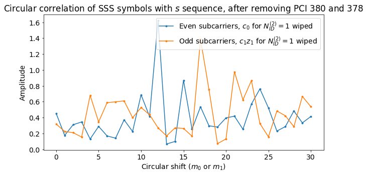
If we remove the contribution of PCI 380 to the first SSS transmission we have received, we can now compute the circular correlations using \(N_{ID}^{(2)} = 0\) in order to detect the sequence for PCI 378. We see that the peaks appear in the same positions as before (because \(N_{ID}^{(1)}\) is the same). However, the amplitude of the peaks is much smaller. In fact, it is necessary to remove the contribution of PCI 380 to detect these peaks, since otherwise they would be below the noise level caused by the cross-correlation with PCI 380.

We remove the contribution of PCI 380 from the templates and wipe the corresponding sequence for PCI 378. The results are shown below. In the right hand side of the plot we can see that the phase follows a steady slope versus frequency, since presumably PCI 378 is stronger than PCI 379 and dominates. In the left hand side the amplitude is smaller and the phase has large jumps as if following a BPSK pattern. This is because now the effect of PCI 379 starts to be seen.

We are interested in using the phase versus frequency slope to measure the group delay of PCI 378 (relative to that of PCI 380). This is something that we could have tried to do with the PSS, but it would have been more difficult, due to the large cross-correlation between \(N_{ID}^{(2)} = 0\) and 2. Before doing this measurement, in order to obtain the best results, we will also estimate PCI 379 and remove its contribution.

Another thing that we can do at this point is to take each of the SSS transmissions, remove the contribution of PCI 380, and wipe the sequence for PCI 378. Then we compute and plot the average across all subcarriers, colouring by beam. The resulting plot is shown below. Each dot corresponds to an individual SSS transmission. We see that we obtain the same kind of pattern as when we estimated the relative complex amplitudes of PCI 378 using the PSS templates. Here we are treating each SSS transmission individually, so this plot shows that the relative phase of PCI 378 and PCI 378 stays consistent in all the transmissions, and depends only on the beam.

If we remove the contributions from PCI 380 and 378 from the first received SSS transmission, we can perform the circular correlations for \(N_{ID}^{(2)}=1\), obtaining the plot below. The peaks corresponding to \(N_{ID}^{(1)} = 126\) are rather weak, but still recognizable.

Now we will estimate the relative complex amplitudes of the contributions of PCI 378 and PCI 379. In the above we have worked with data that had been equalized with the degree 4 polynomials that we fitted to the PCI 380 PSS. Since the channel response given by these polynomials need not match the channel response of PCI 378 and 379, it is better to use the data with the simple equalization we did first (only amplitude, phase and group delay), and consider the degree 4 polynomials only when removing the contribution of PCI 380. For PCI 378 and 379 we will assume a non-dispersive channel with zero group delay relative to this simple equalization.

The templates formed with this simple equalization are shown here. The curvature in the amplitude and phase response that was corrected by the degree 4 polynomials is now visible.

We perform a linear least squares fit to each of the templates using a linear combination of the channel response given by the polynomials (which represents the contribution of PCI 380), the product of the SSS sequences for PCI 378 and PCI 380 (which represents the contribution of PCI 378), and the product of the SSS sequences for PCI 379 and PCI 380 (which represents the contribution of PCI 379).

The complex amplitudes of the terms corresponding to PCI 378 and 379 in this least squares fit are shown below. These indicate the complex amplitudes of PCI 378 and 379 relative to PCI 380. The plot is very similar to the one we obtained with the PSS. This gives us confidence in the fact that we are separating and measuring each of the individual signals correctly, and what we see is not caused by some cross-correlation (as we have arrived to the same result using the PSS and SSS, which have completely different cross-correlation properties).

We can use the results of the least squares fit to remove the contributions of PCI 379 and 380, so as to only leave PCI 378. Then we wipe off PCI 378. This gives a plot that is somewhat cleaner than the one at which we arrived by removing PCI 380 only. In particular, the amplitude is not as wavy.

We can fit a linear slope to the phase of the subcarriers above subcarrier number 30. This slope measures the group delay of PCI 378 relative to PCI 380. Since the slope is negative, this means that PCI 378 is arriving later than PCI 380. The delay is between 180 and 280 ns depending on the template we use to measure (though arguably these estimates are quite noisy).

It would make sense that PCI 378 arrives somewhat later than PCI 380, since the antennas for PCI 378 are farther away from the receiver. The difference in straight-line paths is on the order of 50 metres (167 ns). However, this raises the question of how the transmitters are synchronized. Since the antennas are not in the same location, the synchronization needs to be distributed via cables originating from a common source. I don’t know whether the cable delays are compensated or not. If they aren’t, then the analysis of the delay difference that we see between PCI 378 and PCI 380 would also need to take into account the difference in cable lengths.

Another remark pertains PCI 379. Its signal is much weaker than PCI 378, so I haven’t been able to estimate its group delay. However, we should take into account that we are looking at all these signals at the delay of PCI 380 (we have used the group delay for this PCI to equalize). If a signal has a substantially different delay, then we will see large losses for that signal when averaging all the subcarriers together, when assuming zero delay in a linear fit, or when correlating with the \(s(n)\) sequence.

The antennas for PCI 379 are presumably farther away from the receiver than those for PCI 378 and 380. I think they are located at the north end of the building, which is about 125 m further away. This would give an excess delay of 417 ns (not taking into account the cable delays). This delay is still on the order of 1/2 of the reciprocal of the signal bandwidth (930 kHz), but if the extra cable delays are also on the order of 400 ns, we could see a total delay that starts being comparable to the reciprocal of the signal bandwidth. This would cause large losses if we don’t correct this delay, so it could in part explain why PCI 379 appears so week. A more elaborate approach to detect and estimate the PCI 379 signal would attempt to estimate and correct its group delay, perhaps by performing a blind search over a certain range of delays.

Another technique that we could use is to remove the contribution from the PCI 380 PSS (and maybe PCI 378 also) in the time-domain signal. Then we could attempt to correlate with the three PSS waveforms to see if we get new correlation peaks at other delays. Originally these would have been hidden by the correlation against the PCI 380 PSS. This approach could not only be used to try to see if PCI 379 is present at a substantially different delay, but also to try to detect signals from other cell sites, which would be around 1 km away, and hence present much larger delays.

Other remarks

Another remark about the synchronization of different transmitters is that if we compare the synchronization of the three cells (Orange, Vodafone and Movistar) that can be seen in the recording, Orange and Vodafone transmit with the same synchronization, while Movistar has a different synchronization.

The figure below illustrates this difference. The synchronization signals for the three cells can be seen in the waterfall. We see that the synchronization signals for Orange (bottom cell) and Vodafone (centre cell) start at the same time, while the synchronization signals for Movistar (top cell) starts later. The time difference of ~1290 microseconds is marked with the cursors.

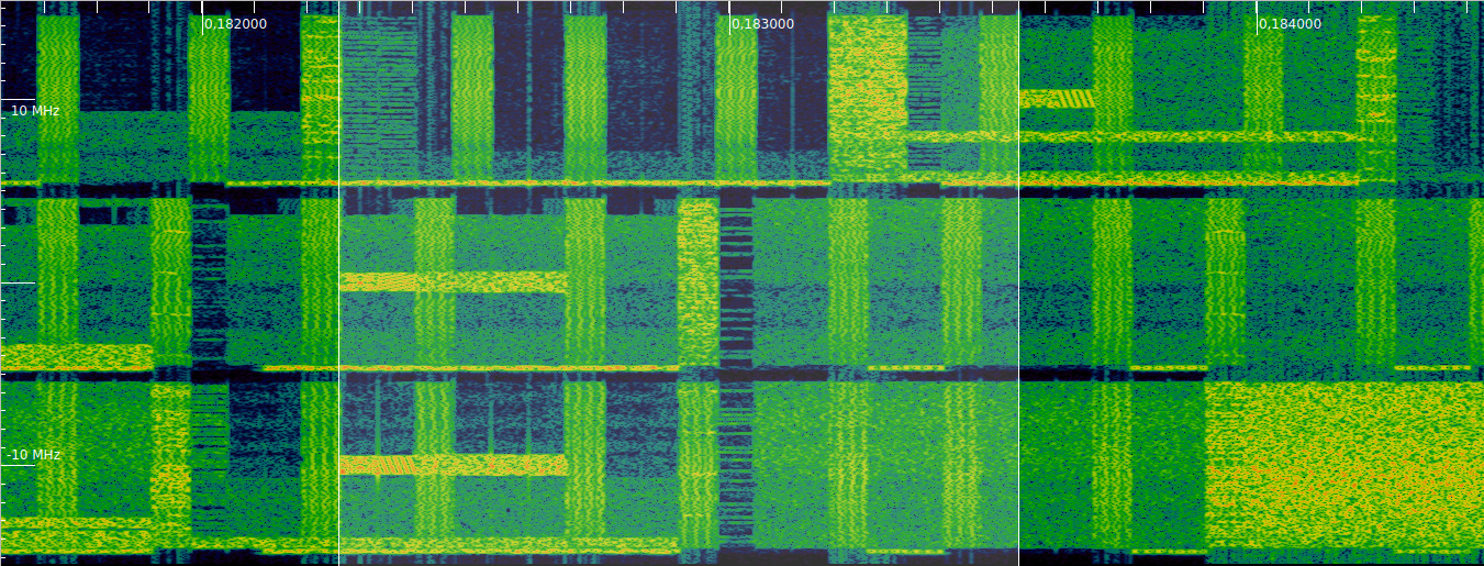
However, a closer look at the waterfall shows that the PBCH follows the synchronization signals of Orange and Vodafone, while in the Movistar signal there is no PBCH transmission after these synchronization signals. This means that there is an additional 5 ms time difference between the radio frames of these cells.

Another thing that we can see directly in this waterfall is the \(N_{ID}^{(2)}\). By looking at the waterfall pattern of the PSS, we can distinguish the three different PSS sequences. We see that the PSS of Orange and Movistar look the same, while the PSS of Vodafone (which we know is \(N_{ID}^{(2)} = 2\)) looks different.

Code and data

The calculations and plots in this post have been done in this Jupyter notebook. The one second excerpt of the LTE downlink recording is the LTE_downlink_806MHz_2022-04-09_30720ksps SigMF recording in this LTE recordings folder.