Timing SDR recordings with GPS

Following a discussion on Twitter about how to use satellite signals to check that distributed receivers are properly synchronized, I have decided to write a post about how to use GPS signals to timestamp an SDR recording. The idea is simple: we do a short IQ recording of GPS signals, and then process those signals to find the GPS time corresponding to the start of the recording. This can be applied in many contexts, such as:

• Checking if the 1PPS synchronization in an SDR receiver is working correctly.
• Timestamping an SDR recording without the need of a GPS receiver or 1PPS input, by first recording GPS signals for some seconds and then moving to the signals of interest (this only works if you’re able to change frequency without stopping the sample stream).
• Measuring hardware delays between the 1PPS input and the ADC of an SDR (for this you need to know the hardware delay between the antenna connector and 1PPS output of your GPSDO).
• Checking if synchronization is repetitive across restarts or power cycles.

We will do things in a fairly manual way, using a couple of open source tools and a Jupyter notebook. The procedure could certainly be automated more (but if you do so, at some point you might end up building a full fledged GPS receiver!). The post is written with a walk-through approach in mind, and besides the usefulness of timestamping recordings, it is also interesting to see hands-on how GPS works.

Recording set up

The procedure that we will follow here can be applied to any IQ recording of the GPS L1 band (1575.42 MHz, with at least 2 MHz bandwidth, ideally 4 MHz or more). Typically you can record from a GPS active antenna directly with an SDR, provided that you can power the antenna with a bias tee.

For this post, in order to demonstrate that the techniques work and ensure that all my calculations are correct, I have made a recording that is synchronized to the 1PPS output from a GPDSO. The recording set up is somewhat interesting by itself, and shows some potential problems that can appear in other synchronization scenarios.

I have used a USRP B205mini, recording at a frequency of 1575.42 MHz and 4 Msps. The RX2 port is connected to the same GPS antenna as the GPSDO using a Wilkinson splitter. Since the B205mini only has a single external reference input that can be used for 1PPS or 10 MHz (but not both), we use it as 1PPS and connect it to the 1PPS output of the GPSDO.

Making this work in GNU Radio is fairly straightforward. We set Sync to “PC Clock on Next PPS” and Mb0 Time Source to “External” in the UHD source block.

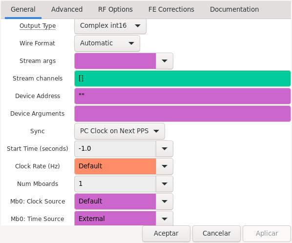
This enables the 1PPS input of the USRP and performs the following synchronization scheme to set the internal time of the USRP. When the USRP is initialized before the flowgraph starts running, the PC keeps polling the USRP until it sees a 1PPS edge. Then it reads the current time from the PC clock, increments by one second, rounds it up to an integer number of seconds, and tells the USRP to latch that value at the next 1PPS edge. Provided that the PC clock is accurate to 0.5 seconds (which in my case is, as I’m using NTP), this will synchronize the USRP correctly.

However, there is a pitfall here. Even though the reference input is used for 1PPS, the USRP also uses it to discipline its internal reference clock. Basically, it counts how many reference clock cycles pass between PPS edges, and uses that to set a DAC that controls the TCXO tune voltage. Depending on what you’re doing, this feature might be useful or annoying.

For recording GPS signals it is rather annoying. The typical processing of GPS signals uses a PLL for tracking the carrier phase. The bandwidth of this PLL is usually between 15 and 40 Hz. The TCXO control done by the USRP makes its local oscillator perform discrete frequency jumps (I think that it jumps every second, which makes sense, since it has to wait for a full second to count). The jumps can be much larger than the PLL bandwidth (specially at the beginning of the recording, when the TCXO frequency error is large), and will make the PLL lose lock when we attempt to process the signal later. If you have some sort of CW carriers in your recording (perhaps you have some that come form interference), it’s easy to tell if this is happening because you can see the frequency jumps in the CW carriers.

I don’t know if there is a proper way to disable this feature. What I’ve done is a workaround that consists in disabling the 1PPS input of the USRP after it synchronized. This can be done with a Python Snippet block like so:

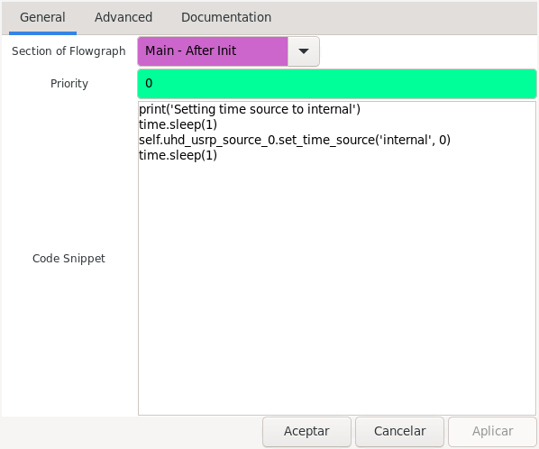
I have found the snippet to be bit hit and miss. Apparently the sleep()‘s help it work better.

This just happens because the B205mini can only have 1PPS or 10 MHz. In many other applications you will have both 1PPS and 10 MHz, and you will not have these problems. Indeed, depending on what you’re doing, having an accurate 10 MHz reference might be essential. Remember that if your reference is 1 ppm off, then your time will drift 1 microsecond every second. So your time synchronization might be very good at the start of your recording, but then it will keep drifting.

The recording I have done is 15 seconds long. In order to read the time from the GPS signal, we need to receive a subframe (GPS transmits the data in 6-second packets called subframes). To have at least one full subframe and some margin, I have chosen 15 seconds. If you already know the time synchronization of your recording with some precision (for instance, better than 10 ms), then it is possible to work with a much shorter recording.

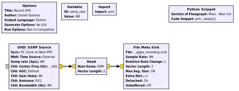
The recording is published in the dataset “Recording of GPS L1 signals” in Zenodo. The flowgraph used to do the recording is in record_gps.grc. The flowgraph looks like this.

Acquisition and tracking using GNSS-DSP-tools

The first step in processing our recording is to acquire the signal of the GPS satellites and track the signal of at least one satellite. To do this, we will use GNSS-DSP-tools, which is a collection of small Python scripts by Peter Monta. These scripts are quite simple and well written, so I suggest anyone interested in the details to check out the code.

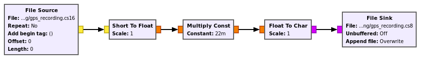
The scripts need the recording in 8-bit IQ format. Since I have done my recording in 16-bit IQ format, I have to convert it with this GNU Radio flowgraph. I have determined the scale factor in order to make good use of the 8-bit range. Since the GPS signals are below the noise floor, the histogram of the samples is a Gaussian. I have tried to set the standard deviation of this Gaussian to be 1/5th of full scale. That still gives some margin to prevent clipping.

First we need to run the acquire-gps-l1.py script to acquire the GPS signals. This will correlate the first 80 ms of the recording against each of the 32 GPS PRNs to try to find what satellites are present in the recording, as well as their Doppler frequency and code phase. The correlation is done in blocks of 1 ms, which are then added non-coherently.

To run this script, we need to indicate it the path to the recording, the sample rate, and the centre frequency for the GPS signals. In our case, since we recorded at 1575.42 MHz, the GPS signals are now at baseband (0 Hz). We run the script and get the following.

$ ./acquire-gps-l1.py GPS-L1-2022-03-27.cs8 4000000 0
prn   1 doppler   600.0 metric  1.58 code_offset  393.4
prn   2 doppler  1800.0 metric  3.19 code_offset  758.8
prn   3 doppler -1200.0 metric  1.65 code_offset 1004.0
prn   4 doppler  1000.0 metric  1.50 code_offset  475.0
prn   5 doppler   800.0 metric  1.61 code_offset  964.8
prn   6 doppler  1800.0 metric  1.54 code_offset  153.4
prn   7 doppler -4200.0 metric  1.53 code_offset  259.5
prn   8 doppler  -200.0 metric  1.53 code_offset  830.4
prn   9 doppler  6800.0 metric  1.49 code_offset  134.6
prn  10 doppler -7000.0 metric  1.58 code_offset  783.7
prn  11 doppler  2400.0 metric  7.22 code_offset  185.8
prn  12 doppler  -200.0 metric  7.98 code_offset  151.6
prn  13 doppler   800.0 metric  1.62 code_offset  881.4
prn  14 doppler -1200.0 metric  1.50 code_offset  123.1
prn  15 doppler -4200.0 metric  1.53 code_offset  813.5
prn  16 doppler  -200.0 metric  1.53 code_offset  285.2
prn  17 doppler  3600.0 metric  1.47 code_offset  940.3
prn  18 doppler  1800.0 metric  1.51 code_offset  860.9
prn  19 doppler  3800.0 metric  1.51 code_offset  421.1
prn  20 doppler  1000.0 metric  1.59 code_offset  956.3
prn  21 doppler -5200.0 metric  1.58 code_offset  438.3
prn  22 doppler  2600.0 metric  5.33 code_offset  465.0
prn  23 doppler -4200.0 metric  1.59 code_offset  272.2
prn  24 doppler  3000.0 metric  1.55 code_offset  605.9
prn  25 doppler  1600.0 metric  6.99 code_offset  425.1
prn  26 doppler -5000.0 metric  1.52 code_offset  149.6
prn  27 doppler -1200.0 metric  1.48 code_offset  404.9
prn  28 doppler  2800.0 metric  1.51 code_offset  128.6
prn  29 doppler  4000.0 metric  1.65 code_offset  603.2
prn  30 doppler -2200.0 metric  1.50 code_offset 1012.0
prn  31 doppler  5200.0 metric  6.86 code_offset  559.7
prn  32 doppler  1000.0 metric  7.18 code_offset  680.3

The metric column indicates the SNR of the acquisition peak. Everything around 1.5 is just noise, while things above 2.0 are definitely GPS signals. We see that satellites G02, G11, G12, G22, G25, G31 and G32 are present in our recording.

We will do the timing analysis using the signal from only one satellite. We choose one of the strongest satellites, and use track-gps-l1.py to track it. Here we will choose G12, since it has the largest metric. The script will produce a plain text output that we can send into a file. The parameters needed by track-gps-l1.py are the same as for acquire-gps-l1.py plus the PRN to track, as well as the Doppler and code offset that the acquisition produced for this satellite (here -200 Hz and 151.6 chips).

./track-gps-l1.py GPS-L1-2022-03-27.cs8 4000000 0 12 \
    -200 151.6 | tee track.txt

The script tracks the signal throughout the 15 seconds of the IQ recording and outputs data to the standard output in a table format. Basically, what this script is doing is correlating the recording with the PRN for G12, while using a DLL to track the code phase and a PLL (a Costas loop, actually) to track the carrier phase (initially an FLL is used to reduce the frequency error). The text output contains IQ dumps produced in the correlator, as well as the state of these tracking loops.

Processing the tracking output

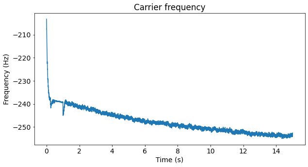
Now we work with the output of track-gps-l1.py in a Jupyter notebook. The notebook can be found here. As a first step, we can plot the carrier frequency of the FLL/PLL to check if tracking was successful. We see that after approximately one second the PLL locks and follows the Doppler of the satellite, plus the receiver clock drift (the error of the SDR frequency reference).

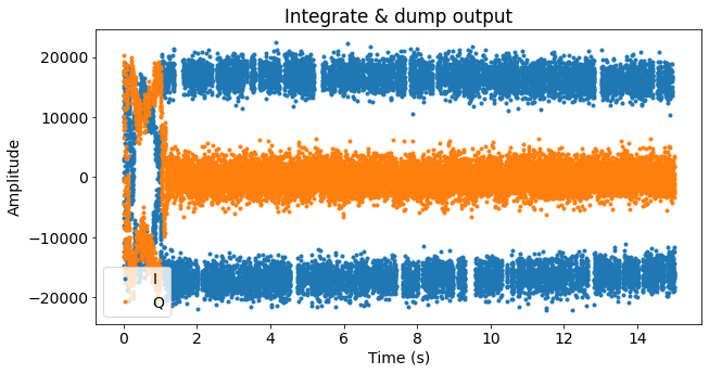
We can also plot the dumps from the integrate & dump correlator. It is producing a dump every 1 ms, corresponding to each repetition of the PRN code (which has 1023 chips and is transmitted at 1.023 Mchip/s). The modulation is BPSK, so after about 1 second the PLL locks and we see that all the signal is in the I component. The BPSK modulation contains data, which we will use to find the time.

GPS transmits its navigation message at 50 symbols per second. Therefore, we have 20 dumps per symbol. We need to determine the offset at which the symbols start. To do this, we consider all the 20 possible offsets, integrate symbol by symbol starting at each offset, and compute the average amplitude. The correct offset will give the maximum amplitude. We use the data between seconds 8 and 12. This is what we obtain.

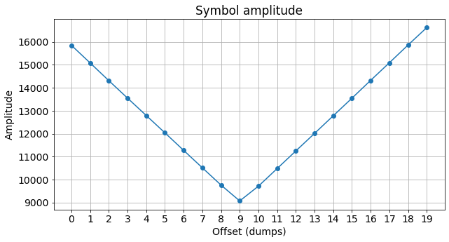
The maximum happens at an offset of 19 dumps, meaning that the first whole symbol in the tracking output starts at dump number 19 (starting to count dumps by 0). With this knowledge, we can now group and average together the 20-dump symbols, obtaining the following.

The beginning of GPS subframes is marked by the 8-bit preamble 10001011. However, it can be a bit tricky to find this preamble correctly, because it is so short that it can appear elsewhere in the data, and moreover it can appear inverted due to the 180º phase ambiguity of the Costas loop PLL.

We obtain the bits by taking the sign of the real part of the symbols, and compute and plot the correlation of the 8-bit preamble with the bits. We get the figure below.

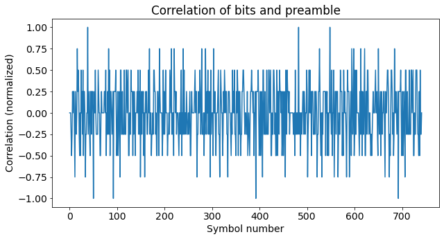
This shows normalized correlation, so a value of +1 (or -1) means that all the 8 bits match.

Since subframes are 300 symbols long (6 seconds), we are looking for several +1 or -1 correlation peaks that are spaced by 300 symbols. Looking at the positions of the peaks, we see that there are -1 peaks at symbols 92, 392 and 692. This means that the first subframe starts at symbol 92. The other correlation peaks should be ignored.

Now we want to read the time information from the subframe. GPS encodes time as a week number (starting at Sunday 6 January 1980) and a time of week (TOW) in seconds. The time of week is transmitted in a 17-bit field in each subframe in 6 second units (since each subframe lasts 6 seconds, this field is basically a counter). This figure from IS-GPS-200M shows the details.

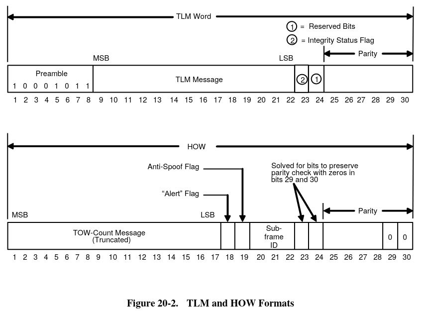
Looking at the TOW of the first subframe, we get 41550 seconds. An important detail is that this TOW refers to the start of the next subframe, so the first subframe actually starts at TOW 41544. It is also a good idea to check the TOW contained in the next subframe to be sure we haven’t messed something up.

Here we will not try to read the week number from the signal. Probably you know in which week you’ve done your recording, but if you really need the week number, it’s also in the GPS navigation message, but not in all the subframes, so you’ll need a recording longer than 15 seconds to guarantee that you see a week number.

Since we know in what dump of the tracking output the first subframe starts, we can compute the TOW corresponding to the first dump of the tracking output by subtracting. This is 41542.141.

Now this gives roughly the timestamp at the start of the recording, except for two things. First, this refers to the time when the signal was transmitted from the satellite. The signal then took between around 60 and 80 milliseconds to arrive to our antenna. We will handle this later. Second, this timestamp is only precise to one millisecond, since we are only counting dumps. To improve the precision we need to look at the code phase of the DLL. This indicates the phase of the PRN code that the tracking script is using to try to match the signal from the satellite. Since the PRN is periodic, this measurement has an ambiguity of one millisecond, but with a good signal it has a precision of a few nanoseconds.

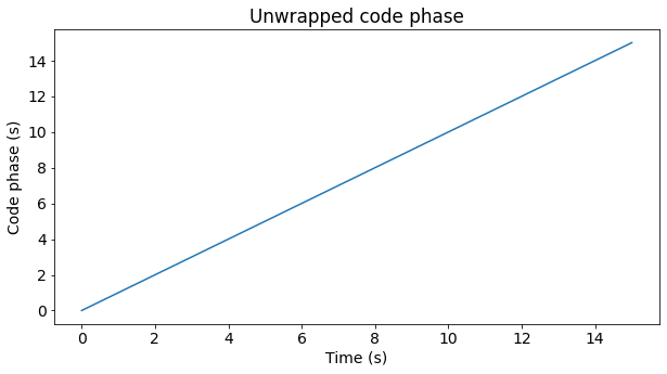
First we look at the unwrapped code phase that track-gps-l1.py generates. We see that the code phase (in seconds) at time \(t\) is quite close to \(t\), so this plot is not so interesting. What happens is that track-gps-l1.py starts counting the unwrapped phase at the start of the PRN repetition that is in course at the beginning of the recording, and then keeps incrementing the code phase each time that the PRN repeats. If the satellite didn’t move and the SDR frequency reference was perfect, then the code phase would change by exactly one second every second. The movement of the satellite and the receiver clock drift make it deviate from this. But the deviation is small enough that we can’t see it in this scale.

Ultimately we are interested in getting the unwrapped code phase at \(t = 0\) (the beginning of the recording). We can’t get it directly because the tracking has started by the code phase we have indicated it (the one we took from the acquisition results). This code phase has a resolution of a few 100 ns, which is too coarse. When the tracking starts, the DLL converges in a few seconds to a much more accurate estimate (the DLL bandwidths that are typically used are 0.5 – 2 Hz).

There are many ways to proceed here. What I’m going to do is to take the code phase data between 5 and 15 seconds (to give time for the DLL to converge), fit a polynomial of degree 2 to this data, and then use the polynomial to extrapolate the correct value of the code phase at time zero. The polynomial of degree 2 models the Doppler frequency (line-of-sight velocity) and the receiver’s reference frequency offset with its degree one term, and the line-of-sight acceleration and frequency drift of the reference with its degree two term. It is not a good idea to fit a higher order polynomial, since the estimate of the higher order terms will probably be too noisy. Also, in some situations it may be enough to use a polynomial of degree one, since the acceleration is not so high (look at the plot of the carrier phase above to get an indication; in this case it changes by about 1 Hz/s).

The figure below shows the difference between the code phase and the degree 2 polynomial we have fitted. The bottom panel is the same data with a different vertical scale so that we can see better what happens after 5 seconds.

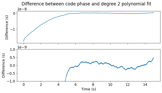
We can see how the initial code phase is wrong by about 20 ns, and how the DLL converges to the correct value. Once the DLL has converged, the jitter it has is a fraction of a nanosecond.

We can now evaluate the polynomial at \(t=0\) to get the estimate of the code phase at the beginning of the recording. As a check, it is worth to check that this code phase, in units of chips, matches the initial code phase that the acquisition indicated, with an error of a fraction of a chip. In our case, the error is about 0.018 chips (one chip is approximately one microsecond, since the chip rate of 1.023 Mchip/s is close to 1 Mchip/s).

Using the code phase at \(t=0\), we can compute that the accurate TOW at the start of the recording is 41542.140148209604 rather than the 41542.141 that we had computed earlier.

Arguably, trying to extrapolate the code phase to the beginning of the recording is not the best idea if we want really accurate results. An alternative idea is, instead of trying to timestamp the beginning of the recording, to timestamp a point in the recording where the DLL has already converged. For instance, \(t = 10\) seconds. In this case, we don’t need to do any extrapolation. We can just do a small linear interpolation to get the code phase at \(t = 10\) (interpolation is needed because none of the instants at which we have code phase measurements will typically coincide exactly with \(t=10\)).

If we are using an accurate 10 MHz reference for our SDR, timing the recording at \(t = 10\) is as good as timing it at \(t = 0\). We can add or subtract 10 seconds to convert between the two. However, if as in my case the SDR reference is not accurate, the timing will have drifted by several microseconds between \(t = 0\) and \(t = 10\).

Another idea if we still want the timing at \(t = 0\) and we don’t have an accurate reference is to track backwards in time, starting from the end of the recording. For this we would have to modify track-gps-l1.py.

Calculating the time of flight of the signal

As we have mentioned, the timestamp we have computed, corresponds to the instant when the signal at the beginning of the recording was transmitted. This signal takes between approximately 60 and 80 ms to travel from the satellite to the antenna. The time that the signal takes to travel is known as time of flight.

Another important detail is that this timestamp is generated by the clock on-board the GPS satellite. This clock is an atomic Cesium clock, so it is quite accurate. However, rather than steering frequently these clocks to keep them close to GPS time, they are often left to drift on their own for long time, so they can accumulate an error of a few milliseconds. This error is known as satellite clock bias.

To make sense of the timestamp 41542.140148209604, which is the time of transmission for G12 at the beginning of the recording, we need to compute the position and clock bias of the satellite at that instant. Then, using the known location for the antenna, we can compute the time of flight.

We will use RTKLIB to do these calculations. RTKLIB is a software toolkit for GNSS positioning that comes with a C API that we can use to do our own calculations. Besides the calculations that I have described, it will also handle for us subtle things such as the Earth rotation correction and the relativistic clock correction.

To do the calculations, we need to know the position of our antenna in ECEF coordinates. This online calculator can be used to convert from latitude, longitude and altitude. This position needs to be accurate if we want to compute an accurate timing solution, so it pays off to use a GPS receiver connected to the same antenna to get its position. In my case, I have taken the position from the GPSDO, which gives latitude, longitude and altitude, and then converted it to ECEF using the calculator. I get the coordinates (in metres) 4840402, -312932, 4128949.

The other piece of data we need is the satellite ephemerides. These give a description of the satellite orbit and clock bias. They can be downloaded from CDDIS. The file that you get needs to match the moment when the SDR recording was done, so if you don’t want to wait a day, the hourly files are useful. In my case I have used hour0860.22n.

I have done a small C application that uses RTLKIB to calculate the time of flight. This time of flight is also corrected with the satellite clock bias, so that the only thing we need to do is to copy the number we get to the Jupyter notebook, and add it to the time of transmission we got.

The interesting part of the code is shown here.

// Compute a first satellite position assuming satellite clock
// bias zero. This is only used to obtain the satellite clock
// bias.
satpos(t, t, satno(SYS_GPS, prn), EPHOPT_BRDC, nav, rs, dts,
       &var, &svh);

// Compute a second satellite position taking into account the
// satellite clock bias
t = timeadd(t, -dts[0]);
satpos(t, t, satno(SYS_GPS, prn), EPHOPT_BRDC, nav, rs, dts,
       &var, &svh);
r = geodist(rs, rr, e);
r -= CLIGHT * dts[0];
printf("Time of flight (corrected with sat clock bias) \
        = %0.12f\n", r / CLIGHT);

We first need to compute the satellite clock bias at the time of transmission of the signal. To do this, we call satpos(), which computes the satellite position and clock bias, because there is not a function in the API to directly calculate the clock bias only. The clock bias is returned in dts[0]. We subtract the clock bias from the time of transmission in order to get the GPS time at the time of transmission, and call satpos() again with the corrected time (the line-of-sight distance can change by up to 700 m/s, so it is important to use the corrected time if we want the best results ).

Finally, we compute the line-of-sight distance, using the receiver position and the satellite position (this is where the Earth rotation correction is applied), and correct it using the satellite clock bias to obtain the “apparent” line-of-sight distance rather than the “true” line-of-sight distance.

To run, the application needs the path to the ephemeris file, the GPS week number (this calendar can be used), the GPS PRN (12 in our case), and the X, Y and Z ECEF coordinates of the receiver’s antenna. I can run it as follows:

$ ./compute hour0860.22n 2203 41542.140148209604 12 \
    4840402 -312932 4128949
Time of flight (corrected with sat clock bias) = 0.074602692582

For simplicity, this small program doesn’t take into account ionospheric and tropospheric delays. The ionospheric delay can be as high as 50-100 ns in certain situations, so depending on the accuracy you need, you might want to correct it. This may be done with RTKLIB and either an IONEX map, which is more accurate, or the Klobuchar model, which is less accurate but only uses data included in the GPS ephemerides. The tropospheric delay is often less than 10 ns.

Final calculations

Now we can go back to the Jupyter notebook and add the time of flight to the time of transmission that we got. We get the following GPS timestamp for the beginning of the recording: 41542.21475090219.

Let us compare this timestamp with the timestamp that UHD has produced using the 1PPS synchronization. We can do the following to read the timestamps in the recording metadata.

gr_read_file_metadata -D GPS-L1-2022-03-27.hdr | less

We see that the first timestamp is

Seconds: 1648380724.2147593125000000

This is the UNIX timestamp at the beginning of the recording. Taking into account that GPS is currently 18 seconds ahead of UTC due to leap seconds being inserted into UTC but not in GPS time, we see that this UNIX timestamp corresponds to TOW 41542.2147593125. Note that besides these 18 seconds, there is a difference between GPS time and UTC, but this difference is usually only a few ns, so typically we will not care about it.

Comparing the GPS timestamp and the UHD timestamp, we see that the UHD timestamp is 8.41 microseconds ahead. I don’t know the details of how the USRP B205mini 1PPS timestamping works at the FPGA level, but in principle I would expect this kind of delay of a few microseconds, due to hardware delays. What probably happens is that when the PPS edge comes, a sample at some point in the FPGA is tagged as corresponding to the PPS. There is some pipelining in the FPGA and in the AD9361, so that particular sample arrived to the ADC some time ago (and we actually care about when the sample arrived to the antenna connector on the USRP, but I think that the analog delay between the antenna connector and ADC is much smaller than the digital delay that comes after). The delay of 8.41 microseconds is equivalent to 33.64 samples at 4 Msps, so it seems quite reasonable as a digital delay (although it’s convenient to mention that some part of the receive chain, particularly near the AD9361 ADC, use oversampling and so run at a higher sample rate).

Another important note is that the beginning of the recording actually happens a couple seconds later from the moment when the PPS synchronization is done (due to the sleeps I put in the code), so the synchronization would have drifted by a couple microseconds by the start of the recording.

Some more thoughts

Here I have shown how to use a single satellite to compute a timestamp, but the recording has several satellites in it. You could use each of the satellites to compute the same timestamp, and then do a weighted average. Or you could even use 4 or more satellites to compute the antenna position and the timestamp. This can be done with RTKLIB, but at this point you’re building a yet more complete GPS SDR receiver, so it’s probably better to get the antenna position from somewhere else.

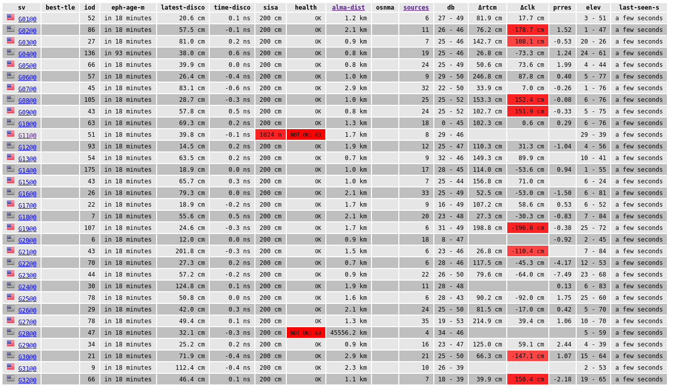
You can also use the different satellites in the recording as a cross-check. In fact, you need to be aware that sometimes satellites are marked as unhealthy and should not be used. Galmon.eu can be used to see in real time the satellite status, and you can also check the official GPS constellation status with the US Cost Guard. For instance, in my case G11 is marked as unhealthy and should not be used, as this screenshot from galmon.eu shows.

In the Jupyter notebook, I have used the small compute application to calculate the time of flight of all the satellites (using the same timestamp for all of them for simplicity, so the results are only approximate), and then checked that the code offsets obtained in the acquisition make sense. These should be accurate to a fraction of a chip. We see that in fact G11 is off by about 2 chips, or 2 microseconds.

Software and data

The recording used in this post is published in the dataset “Recording of GPS L1 signals” in Zenodo. The GNU Radio flowgraphs, Jupyter notebook and C application are in this repository.