Many Amateur radio operators are familiar with the effects of the ionosphere at HF frequencies. However, the effects of the ionosphere are also noticeable at much higher frequencies. In particular, at L band, which is used by most satellite navigation systems. Thus, GNSS receivers can be used to measure ionospheric parameters. These measurements are usually distributed as TEC maps in IONEX files.
Here I describe some basic ionospheric physics, how a GNSS receiver can measure the ionosphere, and give some Python code to study TEC maps in IONEX files. Then I use TEC maps to study the CODAR ionospheric observations I did in December last year.
At VHF and higher frequencies, the ionosphere acts as a dispersive medium, meaning that the index of refraction is frequency dependent. This causes different phase and group velocities in the medium. At these frequencies, the (phase) refractive index of the ionosphere can be approximated by\[n = \sqrt{1-\left(\frac{f_p}{f}\right)^2},\]where \(f\) is the frequency and \(f_p\) is the so called critical frequency, which is the frequency such that for frequencies lower than \(f_p\) a vertically incident wave is reflected by the ionosphere and for frequencies higher than \(f_p\) a vertically incident wave penetrates the ionosphere.
The critical frequency depends on the electron density of the ionosphere. Indeed, it is usual to approximate\[f_p = 8.98\sqrt{N_e},\] where \(N_e\) is the electron density in electrons per \(\mathrm{m}^3\) and \(f_p\) is given in Hz. As anyone familiar with HF propagation knows, for typical values of \(N_e\), the critical frequency lies in the HF band (perhaps around 10MHz).
For frequencies much higher than \(f_p\), the above expression for the refractive index \(n\) can be approximated by the first order Taylor expansion of \(\sqrt{1-x}\) as\[n \approx 1-\frac{1}{2}\left(\frac{f_p}{f}\right)^2 = 1 – 40.32\frac{N_e}{f^2}.\]
When the dispersion is small, the group refractive index, which is defined as \(n_g = \frac{c}{v_g}\), where \(v_g\) is the group velocity, can be computed from the refractive index \(n\) as\[n_g = n + f\frac{dn}{df}.\]In this case, we have\[f\frac{dn}{df} = \left(\frac{f_p}{f}\right)^2\frac{1}{\sqrt{1-\left(\frac{f_p}{f}\right)^2}} \approx \left(\frac{f_p}{f}\right)^2.\]Therefore, using the approximation above for \(n\), we obtain\[n_g \approx 1+\frac{1}{2}\left(\frac{f_p}{f}\right)^2 = 1 + 40.32\frac{N_e}{f^2}.\]
Now consider a signal travelling through the ionosphere, from a satellite to a receiver on the ground. The observed phase delay in seconds is given by\[\delta_p = \frac{1}{c}\int_\gamma n – 1\,dx = -\frac{40.32}{cf^2}\int_\gamma N_e\,dx,\]where \(\gamma\) is the propagation path from the satellite to the receiver. Since \(n\) is close to \(1\), \(\gamma\) can be approximated by the straight line segment between the satellite and receiver. Similarly, the group delay can be computed as\[\delta_g = \frac{1}{c}\int_\gamma n_g – 1\,dx = \frac{40.32}{cf^2}\int_\gamma N_e\,dx = -\delta_p.\]
The quantity\[\int_\gamma N_e\,dx\] is known as the slant total electron content, or STEC. It has units of electrons per \(\mathrm{m}^2\) and it can be thought of as the number of electrons contained in a cylinder whose axis is the straight line segment between the satellite and receiver and whose cross-section has an area of \(1 \mathrm{m}^2\).
To remove the geometry between satellite and receiver, it is usual to consider the vertical TEC or VTEC. This is the STEC for a satellite directly above the receiver, so that the propagation path crosses the ionosphere vertically. A STEC value can be converted to the corresponding VTEC just by multiplying by \(\cos \alpha\), where \(\alpha\) is the incidence angle. This conversion factor comes from a simplified model that assumes that the ionosphere is a thin sell (usually taken at an altitude of around 350km). TEC values are usually given in TEC units or TECU, which correspond to \(10^{16}\) electrons per \(\mathrm{m}^2\).
From the formulas above, we see that a GNSS receiver that is able to calculate phase and group delays at a single frequency or either the phase delays or the group delays at two frequencies can be used to calculate the STEC and then convert to VTEC (which is usually referred to as TEC). More information about the ionosphere in the context of GNSS receivers can be found here.
One of the derived products from the observations of the global network of GNSS monitor stations and receivers are IONEX files, which contain worldwide TEC maps given at fixed intervals. These are used for ionospheric corrections in GNSS observations, but have also many other uses. For instance, TEC maps can be really valuable to understand and judge HF propagation. However, they are relatively unknown among the Amateur radio community.
The relation between the TEC and the critical frequency, say \(f_{o,F2}\), which is more common in HF ionospheric studies is given as follows. The frequency \(f_{o,\mathrm{F2}}\) is related to electron density as above by \(f_{o,F2} = 8.98\sqrt{N_{m,\mathrm{F2}}}\), where \(N_{m,\mathrm{F2}}\) is the maximum electron density in the F2 layer. The parameter \(\tau = \mathrm{TEC}/N_{m,\mathrm{F2}}\), which is called slab thickness of the ionosphere, is a subject of study and there are some models for it. See, for instance, this article. Note that \(\tau\) has units of meters. It can be interpreted by modelling the ionosphere (or rather, the F2 layer) as a shell of thickness \(\tau\) and constant electron density \(N_{m,\mathrm{F2}}\). Usual values for \(\tau\) range between 200 and 600km.
As a rule of thumb, for a slab thickness of 400km, 1 TECU gives a critical frequency of 1.42MHz. Note that the critical frequency scales with the square root of TEC, so 100 TECU give a critical frequency of 14.2MHz.
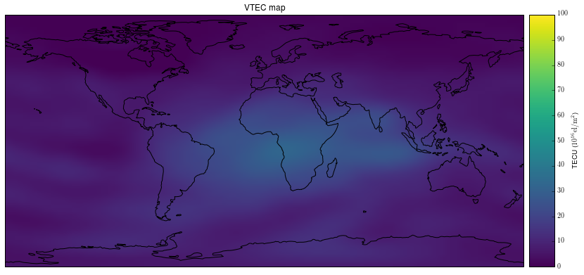
I have made a Jupyter notebook that downloads and parses IONEX files and plots TEC maps. The notebook includes several useful utility functions and some examples. The TEC maps are plotted easily using Cartopy. An example TEC map can be found at the top of this post.
There are also some examples comparing the yearly variation of TEC over Madrid and Sydney throughout the year 2017 to try to observe the winter anomaly in the northern hemisphere.
Finally I have plotted the TEC for the days of my CODAR advent recording to try to see if there is any relation between the TEC values and the qualitative behaviour of the ionosphere observed in the CODAR recording. The CODAR stations recorded are in the north of Spain, so I have plotted the TEC over Valladolid, where single-hop reflections would happen.
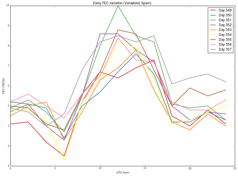
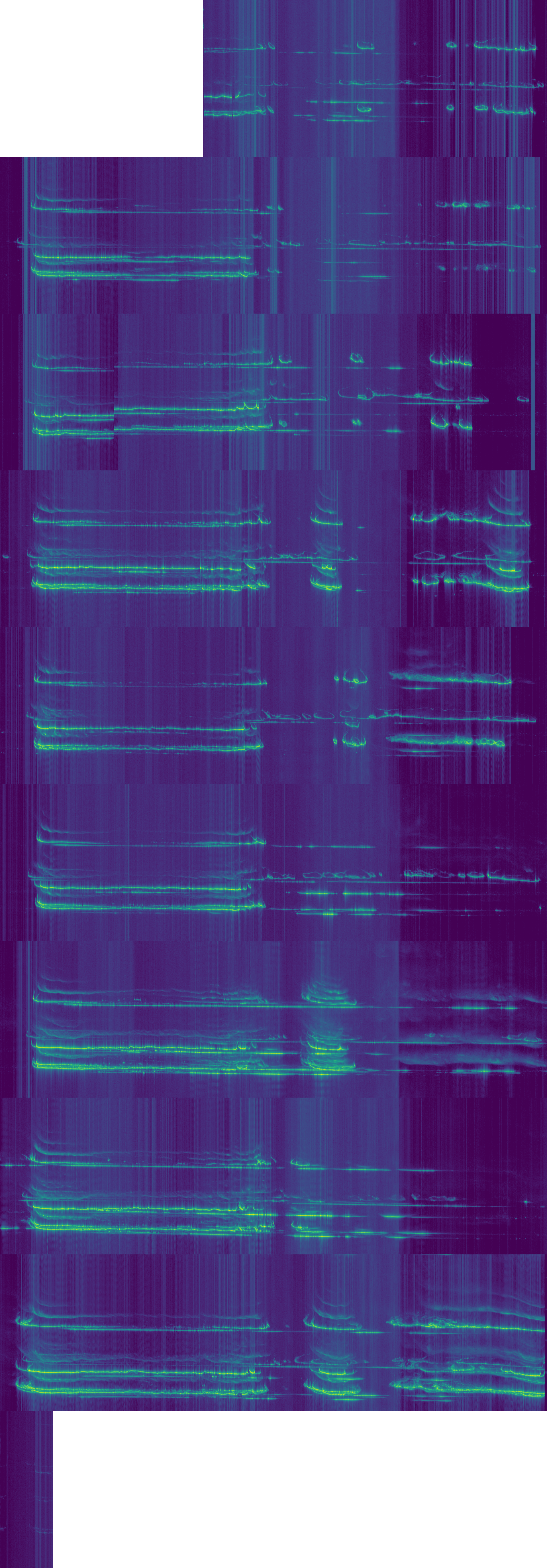
My CODAR advent recording can be seen below. Each of the rows represents one day, starting at day 349. I have noted that days 355 and 357 have unusually high TEC levels at night. These seem to match the CODAR data, in that many strong reflections where received at night during these two days. However, day 352 also has strong reflections at night (albeit they have a rather different shape to those of days 355 and 357), but the TEC level is low. Other than that, I have not seen any other clear matches between the TEC and CODAR data.
Muy interesante. Bien explicado.