A few days ago, Bert Hubert, from galmon.eu noticed that Galileo satellite E24 was somewhat special because it had unusually large BGDs. This raised a number of questions, such as what is the physical interpretation of BGDs, what they have to do with broadcast clock models, and so on.
In this post I will explain a few basic facts about BGDs and related topics, following an approach that is perhaps different to that of the usual GNSS literature, and also study the current values for the Galileo constellation. People who know all the details about the BGDs or who just want to see a few pretty plots can skip all the first section of the post.
The go-to reference for BGDs and any other element of the Galileo Open Service navigation message is the Galileo – Open Service – Signal In Space Interface Control Document (OS SIS ICD V1.3), so here I will try to stick to the notation used there as much as possible. The relevant sections that I will be discussing are 5.1.4 and 5.1.5.
Let’s start from the basics, which will lead us to Equation 12 in the SIS ICD. The whole concept of time in a GNSS constellation is governed through the constellation time scale, which in the case of Galileo is the GST. This is a time reference that doesn’t exist physically, and which is only brought into play by speaking about how real physical clocks differ from this ideal timescale. As such, it is often called a paper clock.
GNSS signals are structured in time, in such a way that to each instant of GST (or the corresponding constellation clock, for other constellations), we have assigned a specific value (actually a voltage amplitude, since the signal is an electromagnetic wave) to each of the particular signals of each satellite in the constellation. If everything was perfect, then the satellites would transmit the corresponding signal at exactly the precise instant according to GST. But the transmissions from each satellite are driven by their own imperfect physical clocks. Thus, there is always a small offset between when the satellite is really transmitting something and when it should be transmitting it according to GST.
The way to write this mathematically is to denote by \(TOT_m\) the scheduled time of transmission according to the constellation clock (so the time when a particular signal should be transmitted if following GST exactly), and by \(TOT_c\) the time when the satellite actually transmits the signal. The two are related by\[TOT_c = TOT_m – \Delta t_{SV},\]where \(\Delta t_{SV}\) is a time-varying quantity that tells us the time offset in this specific satellite’s transmissions (this is often called satellite clock bias). The equation above is Equation 12 in the SIS ICD.
Now, signals corresponding to different frequencies might suffer different delays and end up not being transmitted simultaneously even if ideally they should. We will write\[TOT_c(f) = TOT_m(f) – \Delta t_{SV}(f)\]to express the dependence on the frequency \(f\). Note that we have a different satellite clock bias for each frequency.
GNSS receivers usually work by measuring the signals from different satellites simultaneously as they arrive to the receiver’s antenna. The receiver is able to work out the corresponding \(TOT_m\)’s from the structure of the signals, and forms quantities called pseudoranges which are defined by \[p = TOR – TOT_m,\]where \(TOR\) stands for time of reception according to the receiver clock. For the purposes of this post, we can think that the \(TOR\) is just a common quantity that is used to form the pseudoranges for all the satellites and that it is just an approximation made by the receiver about the time at which the measurement is done (and the precision of this approximation is not really important). We will write\[p(f) = TOR – TOT_m(f)\]to make the dependence on the frequency explicit.
If \(f_1\) and \(f_2\) are two different frequencies (for example, E1 and E5a), then it is possible to form the ionosphere-free combination of the pseudoranges \(p(f_1)\) and \(p(f_2)\), which is defined as\[p(f_1,f_2) = \frac{f_1^2 p(f_1) – f_2^2 p(f_2)}{f_1^2 – f_2^2}.\]Note that this is just a weighted average of \(p(f_1)\) and \(p(f_2)\). This particular choice of weights has the special property that it cancels out the ionospheric delay to a first order of approximation. As such, almost all applications that need precision use this combination. For example, it is used by the ground segment to determine the satellites orbits and clocks. So in many settings it is more natural to think of the ionosphere-free combination rather than of a single frequency.
Now we consider the following weighted averages\[TOT_m(f_1, f_2) = \frac{f_1^2 TOT_m(f_1) – f_2^2 TOT_m(f_2)}{f_1^2 – f_2^2},\]\[TOT_c(f_1, f_2) = \frac{f_1^2 TOT_c(f_1) – f_2^2 TOT_c(f_2)}{f_1^2 – f_2^2},\]and\[\Delta t_{SV}(f_1, f_2) = \frac{f_1^2 \Delta t_{SV}(f_1) – f_2^2 \Delta t_{SV}(f_2)}{f_1^2 – f_2^2}.\]For now this is just notation, but the convenience of this notation will be seen soon. A straightforward calculation shows that\[\begin{split}p(f_1,f_2) &= TOR – TOT_m(f_1,f_2)\\ &= TOR – TOT_c(f_1,f_2) – \Delta t_{SV}(f_1,f_2).\end{split}\]The quantity \(TOR – TOT_c(f_1,f_2)\) has everything a receiver needs to compute its position, or everything that the ground segment needs to compute the satellite orbit, with the advantage that all ionospheric delays have been cancelled out to first order as stated above (but this is a matter for another post). As such, the ground segment actually determines the ionosphere-free satellite clock bias \(\Delta t_{SV}(f_1,f_2)\), and this is also the satellite clock bias that the receivers using ionosphere-free combinations need for their calculations.
Note that \(\Delta t_{SV}(f_1,f_2)\) doesn’t really have a simple interpretation in physical terms, as \(\Delta t_{SV}(f_j)\) did. It is just a weighted average of clock biases that shows up when dealing with the ionosphere combination. Nevertheless, this is the clock bias that is transmitted in the navigation message, as well as the clock bias that is used in SP3 files. The bias \(\Delta t_{SV}(\mathrm{E1},\mathrm{E5a})\) is transmitted in F/NAV, while \(\Delta t_{SV}(\mathrm{E1},\mathrm{E5b})\) is transmitted in I/NAV.
Single frequency users can’t use \(\Delta t_{SV}(f_1,f_2)\) directly. A single frequency user working on \(f_1\) needs a means to obtain \(\Delta t_{SV}(f_1)\) from \(\Delta t_{SV}(f_1,f_2)\). So let us define \(BGD(f_1,f_2)\) as\[BGD(f_1,f_2) = \Delta t_{SV}(f_1,f_2) – \Delta t_{SV}(f_1).\]In this manner, users of \(f_1\) can compute the satellite clock bias they need by\[\Delta t_{SV}(f_1) = \Delta t_{SV}(f_1,f_2) – BGD(f_1,f_2),\]which is Equation 15 in the SIS ICD.
Now let us work out what \(BGD(f_1,f_2)\) actually is. Expanding the definition of \(\Delta t_{SV}(f_1,f_2)\), we get\[\tag{A}BGD(f_1, f_2) = \frac{\Delta t_{SV}(f_1) – \Delta t_{SV}(f_2)}{\left(\frac{f_1}{f_2}\right)^2 – 1}.\]Now, this is almost Equation 14 in the SIS ICD, which is\[BGD(f_1, f_2) = \frac{TR_1 – TR_2}{1 – \left(\frac{f_1}{f_2}\right)^2},\]where \(TR_1\) and \(TR_2\) are the group delays of the signals at frequencies \(f_1\) and \(f_2\).
This requires a small remark regarding group delays. In a GNSS satellite, there is an atomic clock that controls the generation of the RF signals, then these signals are delayed to some extent as they travel through the satellite payload, and then they are radiated from the antenna. Now, we don’t care about the delays of the signals per se. We only care about differences of delays. In fact, a delay that affects all the signals in the same way is indistinguishable from an atomic clock that is running a bit late. So actually we can’t measure the delays themselves, but only their differences. Under this perspective, Equation 14 makes sense, because it only depends on the difference \(TR_1 – TR_2\).
If we have two signals that should be transmitted simultaneously, so that \(TOT_m(f_1) = TOT_m(f_2)\), but are delayed differently so that they are radiated at different times \(TOT_c(f_1)\) and \(TOT_c(f_2)\), their difference of delays is\[\begin{split}TR_1 – TR_2 &= TOT_c(f_1) – TOT_c(f_2) \\ &= -\Delta t_{SV}(f_1) + \Delta t_{SV}(f_2).\end{split}\]This shows that (A) above is equivalent to Equation 14.
Another important question is what happens with single frequency users that work with \(f_2\). A simple calculation shows that the conversion they need to apply can be computed as\[\begin{split}\Delta t_{SV}(f_1,f_2) – \Delta t_{SV}(f_2) &= \frac{f_1^2}{f_1^2 – f_2^2}\left( \Delta t_{SV}(f_1) – \Delta t_{SV}(f_2) \right) \\ &= \left(\frac{f_1}{f_2}\right)^2 BGD(f_1,f_2).\end{split}\]So users of \(f_2\) compute the satellite clock bias as\[\Delta t_{SV}(f_2) = \Delta t_{SV}(f_1,f_2) – \left(\frac{f_1}{f_2}\right)^2 BGD(f_1,f_2).\]
So to summarise, we may say that \(BGD(f_1, f_2)\) is the conversion from the ionosphere-free satellite clock bias to the single frequency satellite clock biases, scaled in such a way that it can be directly applied to obtain the clock for \(f_1\) (so it needs to be scaled appropriately to obtain the clock for \(f_2\)).
Now let us pass to the study of the BGDs and related quantities for the current Galileo constellation. The work shown here can be seen in this Jupyter notebook. I have focused the analysis on GPS week 2109, which started on 2020-06-07, just because it is a recent week, but old enough so that all final GNSS products have already been released.
First we study the BGDs contained in the navigation message. The I/NAV pages contain the BGD for E1-E5b, and the F/NAV pages contain the BGD for E1-E5a. I have used the BRDM MGEX merged ephemeris products. These are loaded with georinex. Since the BGD depends only on internal delays in the satellite payload, which can change with age, temperature, etc., but are otherwise more or less constant, it varies very little.
The figure below shows the average BGDs for each satellite over the whole week 2109, and small error bars which correspond to the standard deviation (in this post all the plots will have error bars). I have ignored the eccentric satellites E14 and E18.

We see what already Bert had noted. E24 has much larger BGDs than the other satellites. Additionally, the difference between its E1-E5a and E1-E5b BGDs is much larger than for all the other satellites.
As we have seen, the BGDs are very related to the clock models \(\Delta t_{SV}\). Indeed, if we consider three frequencies \(f_1\), \(f_2\), \(f_3\), we have\[BGD(f_1, f_2) – BGD(f_1, f_3) = \Delta t_{SV}(f_1, f_2) – \Delta t_{SV}(f_1, f_3),\]since the \(\Delta t_{SV}(f_1)\) terms cancel out. As the BGDs vary slowly, we can just look at the constant term of \(\Delta t_{SV}\), which is called \(a_{f0}\) and study\[a_{f0}(f_1,f_2) – a_{f0}(f_1, f_3).\]These clock model coefficients are broadcast in the navigation message and their difference should be approximately the same as the difference between BGDs.
The figure below compares the difference between BGDs with the difference between \(a_{f0}\) terms, averaged over one week. As before, the error bars correspond to the standard deviation. There are a few satellites with large error bars on the \(a_{f0}\) differences. These correspond to problems in the consistency of the clock models for E1-E5a and E1-E5b (the difference between clock models should be almost constant, so its standard deviation should be pretty small).
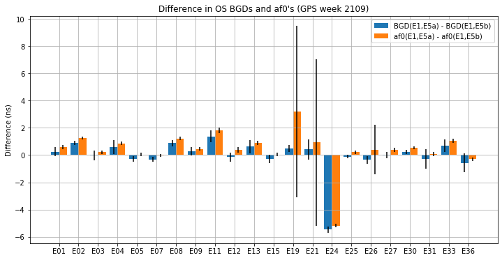
Besides these large error bars for some satellites, we see good agreement between the BGD and \(a_{f0}\) differences. We also note that E24 has a relatively large difference. This actually means that there is a significant delay difference between the E5a and E5b signals, so users of the E5 AltBOC signal might need to take this into account. (Update 2020-07-04: This remark about the delay difference between E5a and E5b is not correct. See the next post).
So far we have only looked at broadcast ephemeris parameters, but these also have their equivalent “precise products” (in the same way that SP3 files are the precise equivalent to broadcast orbits). The DCBs, or differential code biases, are precise products that describe the observed delay differences between pairs of signals. I have used the DCBs from the Chinese Academy of Sciences in Wuhan corresponding to GPS week 2109. These are read with some ad-hoc Python code and plotted here.
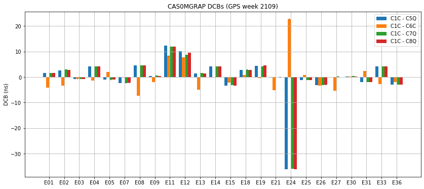
I’m using pilot signals (there are also DCB’s for the C*X signals, which are the combined data+pilot signals). The nomenclature used in DCB files is the one of RINEX files, so C1C stands for the E1C pilot signal, C5Q stands for the E5a-Q pilot signal, C6C stands for the E6C pilot signal, C7Q stands for the E5b-Q pilot signal, and C8Q stands for the AltBOC E5 pilot signal.
We see that, as expected, E24 has the largest biases (also for E1-E6). Note that the sign of the BGDs is opposite to that of the DCBs just because the \(1 – (f_1/f_2)^2\) term in Equation 14 of the Galileo SIS ICD is negative, since \(f_1 > f_2\). Also, the DCBs are directly the difference of delays \(TR_1 – TR_2\), while the BGDs are scaled by \(1/(1 – (f_1/f_2)^2)\).
To check the quality of the broadcast BGDs, we can scale them appropriately and subtract them from the DCBs. The results are shown below. We note that the difference is small, and often zero belongs to the error bars, so we can say that the Galileo broadcast BGDs are in good accordance with the precise DCB products.

So in summary, I have three conclusions for this post:
- The BGDs of Galileo Open Service are accurate enough, and in good agreement with the precise DCBs.
- The satellite E24 is somewhat strange, but that’s all: its data is correct and consistent.
- The broadcast \(a_{f0}\) clock terms for I/NAV and F/NAV are often consistent, in the sense that their difference is almost constant, and very similar to the BGD difference. However, there are occasional problems that might be interesting to study in more detail.
Hi, I was trying to fetch the git annex data for this and the notebooks. Is your annex database still available? It did not work says the linked files do not exist. Looking at the 2 char annex object paths of the links suggest the paths are wrong/gone. All the annex objects are indexed by 3 char now.
Let me know if they are still available (same for svn49).
Thank you,
Robert
Hmm…Let me think about it and look. I did a sparse check out of only those 2 notebooks. Doing: git annex sync eala –content seems to be fetching the data…curious. (some of the BGDs/data rinex files are coming in…)
Thanks,
rfm
Great to see that git annex is working correctly (I rarely tested it). In the worst case I guess that the same files can also be obtained from MGEX (but it’s cumbersome to search them).
I tested git annex again by doing a clean clone on another machine, I it worked fine. I did:
Yes! thank you. I worked through your BGD example. We (@JPL) are looking to recent BGD noise level changes over the last year and earlier. Very nice write-up.
NB: I had a very strange issue in that the file glob(*.rnx) was not sorted! (macOS, py3.11) Took me a while to figure out why the af0_e5a.times were all leading to strange wrap arounds in the interp plots! Finally figured it out by looking at the time(datetime) series and seeing the jumps (all at day boundaries was key signature)…Just for anyone that might run into it!
Best, Robert…
Oh, yes. The output of glob is not sorted alphabetically. It is in the order in which the files “appear on the filesystem”, which can be somewhat random. I usually run the output of glob through sorted(list(…)) because of this. I see that in this case I forgot, and it worked for me, perhaps because I had downloaded the files in order.