The well known Arecibo observatory, besides being used as a radiotelescope and planetary radar, has a powerful HF transmitter that is used to artificially excite the ionosphere, in order to study ionospheric effects using 430MHz incoherent scatter radar. More information about this can be found in the HF proposals page of the observatory web, and in this poster that details the characteristics of the HF facilities.
The HF transmitter has a power of up to 600kW and can use the frequencies 5.1MHz and 8.175MHz. At those frequencies, the dish has a gain of 22dB (13º beamwidth) and 25.5dB (8.5deg) respectively, so the power that is beamed up to the ionosphere is huge. The 430MHz incoherent scatter radar is even more powerful, with up to 2MW. For an introduction to ionospheric incoherent scatter radar, see this lecture by Juha Vierinen, which explains why such huge powers are needed, due to the very weak radar return of ionospheric plasma.
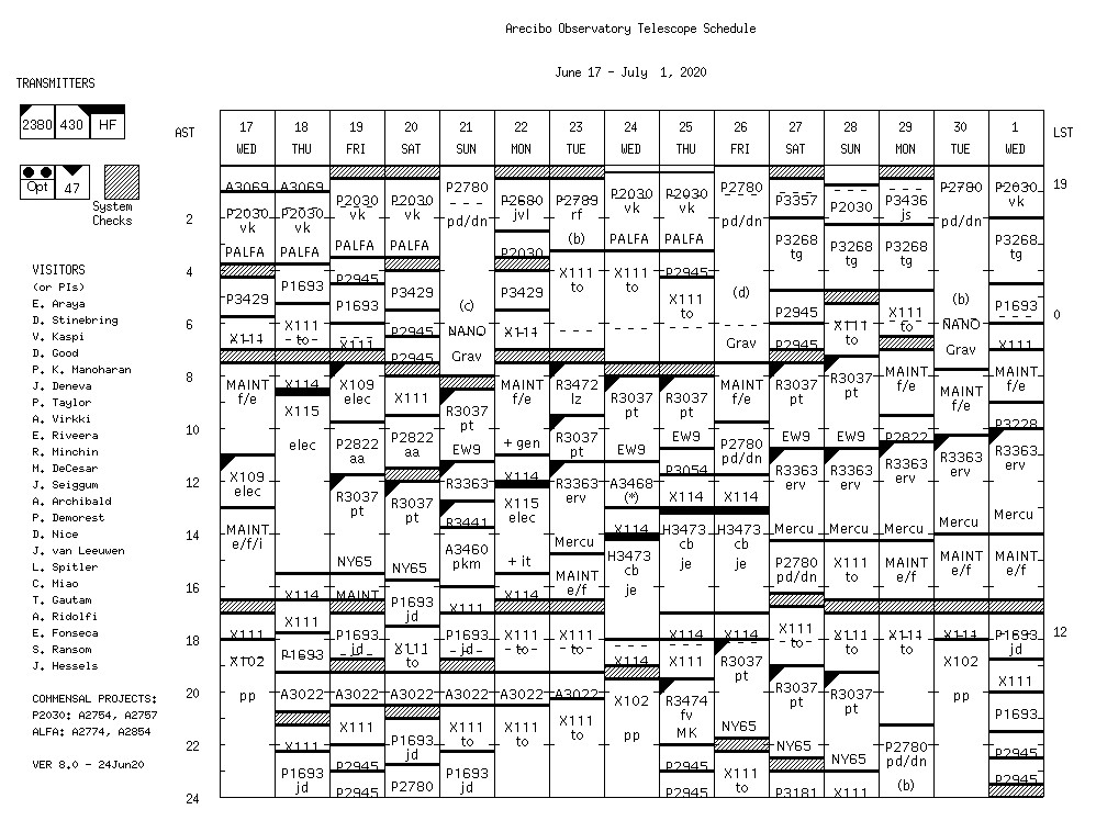
A few days ago, on Wednesday 24, Chris Fallen tweeted that the Arecibo transmitter was active at 5.1MHz. According to the telescope schedule, which can be seen in the figure below (click on the image to view it in full size), there was an experiment that involved the HF transmitter on 2020-06-24 from 18:00 to 22:00 UTC, on 2020-06-25 from 17:00 to 21:00 UTC, and on 2020-06-26 from 17:00 to 21:00 UTC.
I saw Chris’ tweet a few hours too late, but I still could fire up my HF receiver (which consists of a Hermes-Lite 2 and a wire antenna of approximately 15 metres long) at around 21:00 UTC and receive the signal from Arecibo. Then I decided to record the rest of the experiment, and I also did recordings during the next days.
The project associated to this HF experiment is H3473 and its description can be read here. The description is very brief but says that this is an experiment by Fourth State Communications, which is a small company that develops an Enhanced Thermo-Scatter System for ionospheric communications. They claim up to 200Mbps at 2000 miles distance. Pretty impressive.
Since I was a bit informal in doing these recordings, I didn’t take the exact start times and on two days I started after the beginning of the experiment. In all the three days my recordings ended after the experiment stopped. These are the approximate start times for the recordings I made (I have more uncertainty in the first one, the other two should be accurate to one minute):
- 2020-06-24 21:00 UTC
- 2020-06-25 17:21 UTC
- 2020-06-26 16:51 UTC
I have published these recordings as a dataset in Zenodo, for anyone interested in having a look.
The waterfall corresponding to the three days of experiment can be seen below. I have lined up the three recordings by time of day. The resolution of this waterfall is 4.096 seconds and 61mHz per pixel. The total frequency span that is shown is 30Hz, centred on 5100005Hz. You can click on the image to view it in full size.
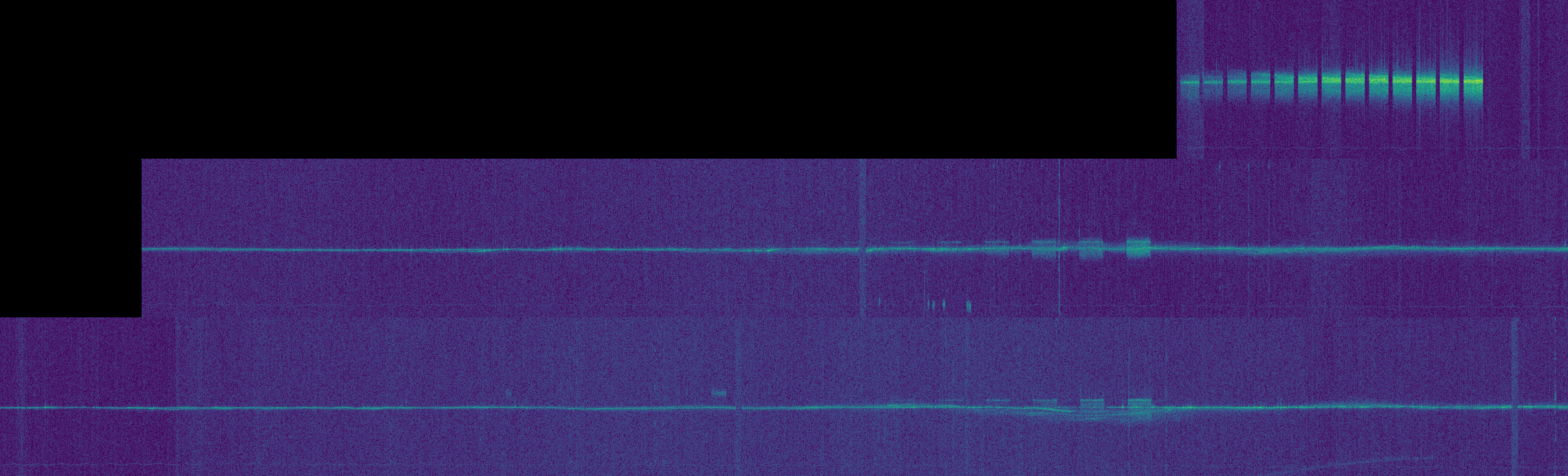
On the first day, the HF transmitter duty cycle was 4 minutes on and 1 minute off. On the second and third day there was a constant CW carrier interfering on the frequency, and the Arecibo signal was much weaker. The duty cycle was different: 5 minutes on and 5 minutes off.
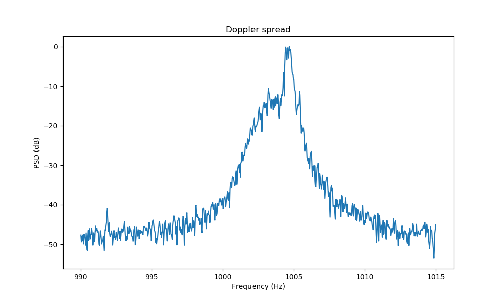
It is interesting to see the Doppler spread on the Arecibo signal and how it changes with time. The figure below shows the power spectral density corresponding to the last transmission on 2020-06-24. We can see a stronger concentrated tone at higher frequency, which is typical in all the three days of experiment, and then weaker signal spreading downwards in frequency.