hf – Daniel Estévez

Waterfalls from the December 2021 eclipse frequency measurement

The HamSci Ham Radio Scienze Citizen Investigation community organized earlier this month the December 2021 Eclipse Festival of Frequency Measurement. The goal of this activity was to measure the frequency of HF time signals such as WWV and RWM over the course of ten days. The experiment lasted from December 1 to December 10, so it included the total eclipse over Antarctica of December 4, which happened between 5:29 and 9:37 UTC.

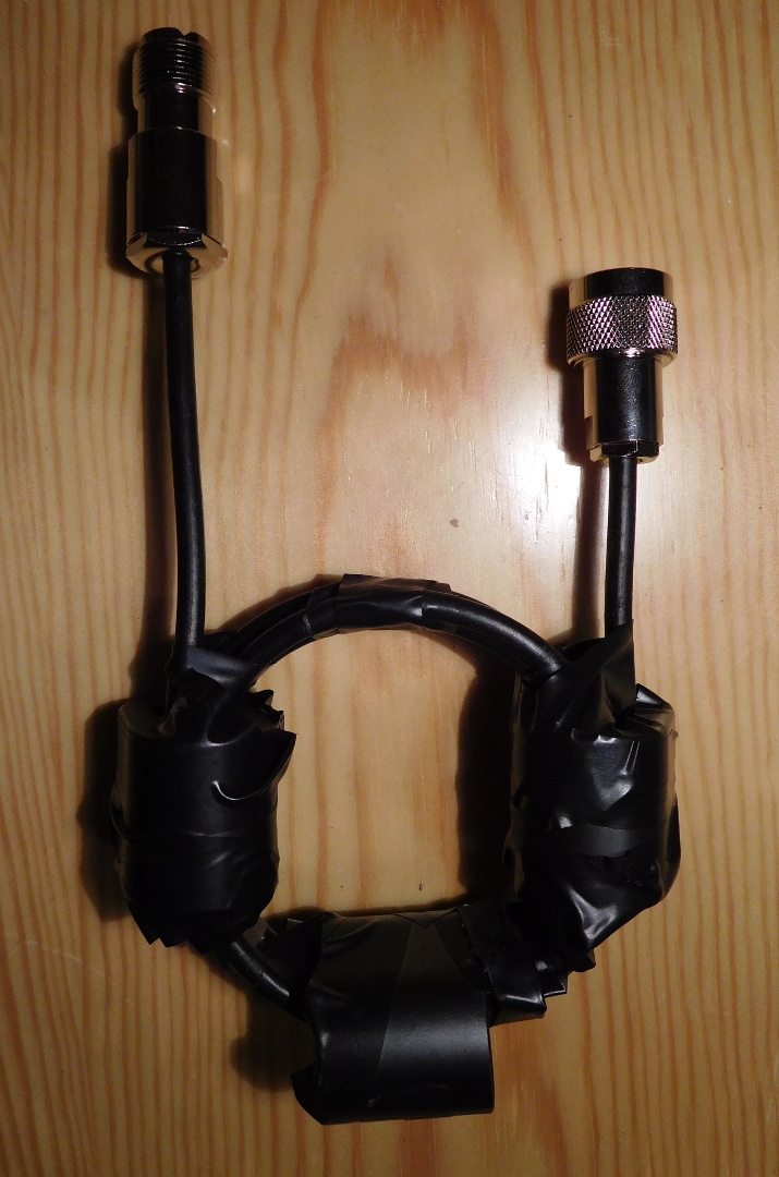
I participated in this activity with my HF station, which consists of a Hermes-Lite 2 beta2 DDC/DUC SDR transceiver and an end-fed random wire antenna about 17 metres long. I used a 10 MHz reference from a GPSDO as described in this post to lock the Hermes-Lite 2 sampling clock. Instead of measuring frequency in real time, I recorded IQ data at 200 sps for the WWV carrier at 5000, 10000 and 15000 kHz and for the RWM carrier at 4996, 9996 and 14996 kHz, so that the data could be post processed later with any kind of algorithms. I have published my recordings in the “December 2021 Eclipse Festival of Frequency Measurment IQ recording by station EA4GPZ” dataset in Zenodo.

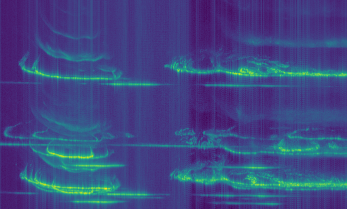
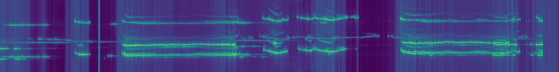
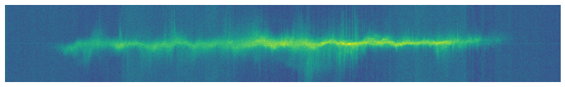
In this post I process the IQ recordings to produce waterfalls that give us an overview of the data. The frequency measurement will be done in a later post.

Receiving Arecibo in HF

The well known Arecibo observatory, besides being used as a radiotelescope and planetary radar, has a powerful HF transmitter that is used to artificially excite the ionosphere, in order to study ionospheric effects using 430MHz incoherent scatter radar. More information about this can be found in the HF proposals page of the observatory web, and in this poster that details the characteristics of the HF facilities.

The HF transmitter has a power of up to 600kW and can use the frequencies 5.1MHz and 8.175MHz. At those frequencies, the dish has a gain of 22dB (13º beamwidth) and 25.5dB (8.5deg) respectively, so the power that is beamed up to the ionosphere is huge. The 430MHz incoherent scatter radar is even more powerful, with up to 2MW. For an introduction to ionospheric incoherent scatter radar, see this lecture by Juha Vierinen, which explains why such huge powers are needed, due to the very weak radar return of ionospheric plasma.

A few days ago, on Wednesday 24, Chris Fallen tweeted that the Arecibo transmitter was active at 5.1MHz. According to the telescope schedule, which can be seen in the figure below (click on the image to view it in full size), there was an experiment that involved the HF transmitter on 2020-06-24 from 18:00 to 22:00 UTC, on 2020-06-25 from 17:00 to 21:00 UTC, and on 2020-06-26 from 17:00 to 21:00 UTC.

WSPR with the LimeRFE

A few days ago, I received a LimeRFE from Andrew Back of Lime Microsystems. He was kind enough to send me a unit so that I can test it and make some usage demos during the ongoing crowdfunding campaign at Crowd Supply.

The LimeRFE is intended to work as an RF frontend for the LimeSDR family, although it can work coupled with any other SDR or conventional radio. As such, it has power amplifiers, filters and LNAs designed to cover the huge frequency range of these SDRs. It is designed to cover all the Amateur radio bands from HF up to 9cm, and a few cellular bands.

As anyone will know, designing broadband RF hardware is often quite difficult or expensive (Amateur radio amplifiers and LNAs are usually designed for a single band), so packing all this into a single unit is a considerable feat. The output power on most bands is around a couple watts, which is already enough for many experiments and applications. The block diagram of the LimeRFE can be seen below.

In this post I show a brief overview of the LimeRFE and demonstrate its HF transmission capabilities by showing a WSPR transmitter in the 10m band, using a LimeSDR as the transmitter.

An overview of IARU R1 interim meeting proposals

The IARU R1 interim meeting is being held in Vienna, Austria, on April 27 and 28. This post is an overview of the proposals that will be presented during this meeting, from the point of view of the usual topics that I treat in this blog.

The proposals can be found in the conference documents. There are a total of 64 documents for the meeting, so a review of all of them or an in-depth read would be a huge work. I have taken a brief look at all the papers and selected those that I think to be more interesting. For these, I do a brief summary and include my technical opinion about them. Hopefully this will be useful to some readers of this blog, and help them spot what documents could be more interesting to read in detail.

Studying IONEX files

Many Amateur radio operators are familiar with the effects of the ionosphere at HF frequencies. However, the effects of the ionosphere are also noticeable at much higher frequencies. In particular, at L band, which is used by most satellite navigation systems. Thus, GNSS receivers can be used to measure ionospheric parameters. These measurements are usually distributed as TEC maps in IONEX files.

Here I describe some basic ionospheric physics, how a GNSS receiver can measure the ionosphere, and give some Python code to study TEC maps in IONEX files. Then I use TEC maps to study the CODAR ionospheric observations I did in December last year.

Analysis of my Hermes-Lite 2 bandscope recording

A few weeks ago I posted how I make wideband recordings of bandscope data with my Hermes-Lite 2. In that post, I sort of promised to do a small analysis of the waterfall I showed. After being busy with other things (PicSat’s launch among them), I’ve finally had time to write something up.

A CODAR advent

Over the last few days, I have been recording CODAR on 4463kHz to produce images of the ionosphere. I started on Friday 15th and the plan was to leave the recording running until Christmas Day, thus producing some kind of “CODAR advent” images. Unfortunately, there seems to be a problem when the receiver runs for several days that results in the sudden loss of the CODAR signal. This problem can be seen at the bottom of the image below. Thus, I have finished the recording on the morning of the 24th. The equipment and software used is the same that I detailed in a previous post.

Using CODAR for ionospheric sounding

CODAR is an HF radar used to measure surface ocean currents in coastal areas. Usually, it consists of a chirp which repeats every second. The chirp rate is usually on the order of 10kHz/s, and the signal is gated in small pulses so that the CODAR receiver can listen between pulses. The gating frequency can be on the order of 1kHz.

CODAR can be received by skywave many kilometers inland. Being a chirped signal, it is easy to extract the multipath information from the received signal. In this way, one can see the signal bouncing off the different layers of the ionosphere, and magnificent pictures showing the changes in the ionosphere (especially at dawn and dusk) can be obtained. For instance, see these images by Pieter Ibelings N4IP, or the image at the top of this post, which contains 48 hours worth of CODAR data.

Here I describe my approach to receiving CODAR. It uses GNU Radio for most of the signal processing, and Python with NumPy, SciPy and Matplotlib for plotting.

Building a feedline HF choke

My current HF antenna is a long wire (around 15 or 20m) connected to an MFJ-993BRT outdoor automatic antenna tuner. The tuner is fed with around 25m of M&P Airborne 10 coaxial cable which runs into the shack. When I installed this antenna, I suffered from high RF currents on the outside of the coax shield when transmitting. These currents go into the shack trying to find a path to earth, since this kind of antenna needs good grounding. Also, while receiving, the coax carried lots of interference into the antenna, especially in the lower bands.

I tried to mitigate this problem by installing a ground rod besides the tuner. This is 2m a copper tube with 50cm buried in the ground. The top of the tube is connected to the tuner ground with a short cable. After installing the ground rod, approximately half of the RF current flowed into the ground rod and the remaining half kept flowing into the shack via the coax shield.

To measure RF current, I have been using a clamp on meter. My design is similar to the design by Ian GM3SEK, but I measure voltage across the output capacitor with a multimeter instead of using a resistor and ammeter coil.

Now I have built and installed a feedline choke following the design of the mid-bands choke by GM3SEK. I use 4 turns of M&P Airborne 5 coax through 3 Fair Rite 2643167851 material 43 cores, wound as an 85mm coil. The finished choke can be seen below.

I have measured the performance of the choke using my Hermes-Lite2 beta2 in VNA mode, as I already did with my mains choke. The results are shown below.

The performance seen in these graphs matches the performance measured by GM3SEK in his document. The choke has a resistance of over 1000 ohms on most of the Amateur HF bands, and up to 5000 ohms in the middle bands.

I have installed the choke directly on the input of the tuner. The RF current flowing on the outside of the coax shield has now decreased to around 2% in several cases and 10% in the worst case. The interference received in the lower bands has also decreased noticeably.

WSPR reports frequency distribution experiment: 20m

Last week I did an experiment where I transmitted WSPR on a fixed frequency for several days and studied the distribution of the frequency reports I got in the WSPR Database. This can be used to study the frequency accuracy of the reporters’ receivers.

I was surprised to find that the distribution of reports was skewed. It was more likely for the reference of a reporter to be low in frequency than to be high in frequency. The experiment was done in the 40m band. Now I have repeated the same experiment in the 20m band, obtaining similar results.