The HamSci Ham Radio Scienze Citizen Investigation community organized earlier this month the December 2021 Eclipse Festival of Frequency Measurement. The goal of this activity was to measure the frequency of HF time signals such as WWV and RWM over the course of ten days. The experiment lasted from December 1 to December 10, so it included the total eclipse over Antarctica of December 4, which happened between 5:29 and 9:37 UTC.
I participated in this activity with my HF station, which consists of a Hermes-Lite 2 beta2 DDC/DUC SDR transceiver and an end-fed random wire antenna about 17 metres long. I used a 10 MHz reference from a GPSDO as described in this post to lock the Hermes-Lite 2 sampling clock. Instead of measuring frequency in real time, I recorded IQ data at 200 sps for the WWV carrier at 5000, 10000 and 15000 kHz and for the RWM carrier at 4996, 9996 and 14996 kHz, so that the data could be post processed later with any kind of algorithms. I have published my recordings in the “December 2021 Eclipse Festival of Frequency Measurment IQ recording by station EA4GPZ” dataset in Zenodo.
In this post I process the IQ recordings to produce waterfalls that give us an overview of the data. The frequency measurement will be done in a later post.
The data was recorded using the hl2_freq_hf.grc flowgraph, which is shown below.
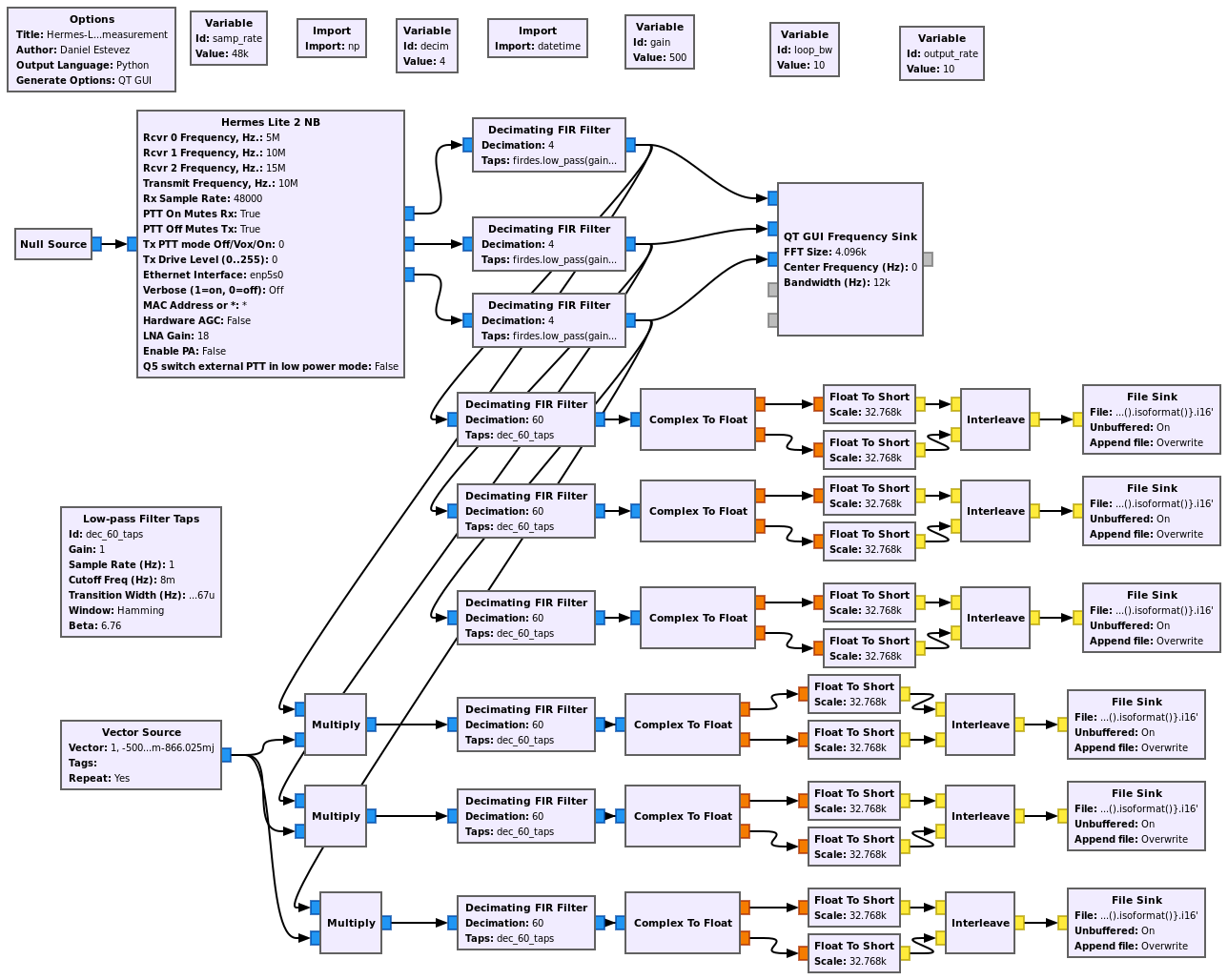
Three FPGA receivers are used in the Hermes-Lite 2, tuned to 5, 10 and 15 MHz. The receivers use 48 ksps IQ. The data for WWV is obtained directly by lowpass filtering. The data for RWM is obtained by mixing with a vector source that contains a periodic complex exponential. Using a vector source instead of a signal source to generate this exponential avoids any frequency errors due to rounding. The IQ data is recorded using 16 bit integers. After recording, the files were converted to SigMF format.
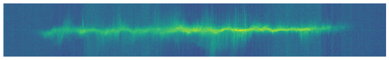
The waterfalls are computed with this make_waterfalls.py Python script. It uses an 8192 point FFT with a Blackman window to compute the spectra, saving only the bins corresponding to the central +/-5 Hz, which is enough for the analysis of the carrier. The time resolution is therefore 40.96 seconds, and the frequency resolution is 24.4 mHz. The mHz level frequency errors due to the FPGA NCO resolution (see this post) have not been corrected, since they are an order of magnitude below the FFT resolution. The waterfalls are saved to npy files.
The waterfall files are read and plotted in this Jupyter notebook. The plots are organised by rows, with each row corresponding to 24 hours aligned to the UTC days, since the propagation follows a daily pattern. There is one plot for each of the 6 signals (3 WWV frequencies and 3 RWM frequencies) that have been recorded. The power scale in all the plots is the same, and encompasses a total range of 80 dB. This allows us to see how the noise floor power decreases when going to the higher frequencies.
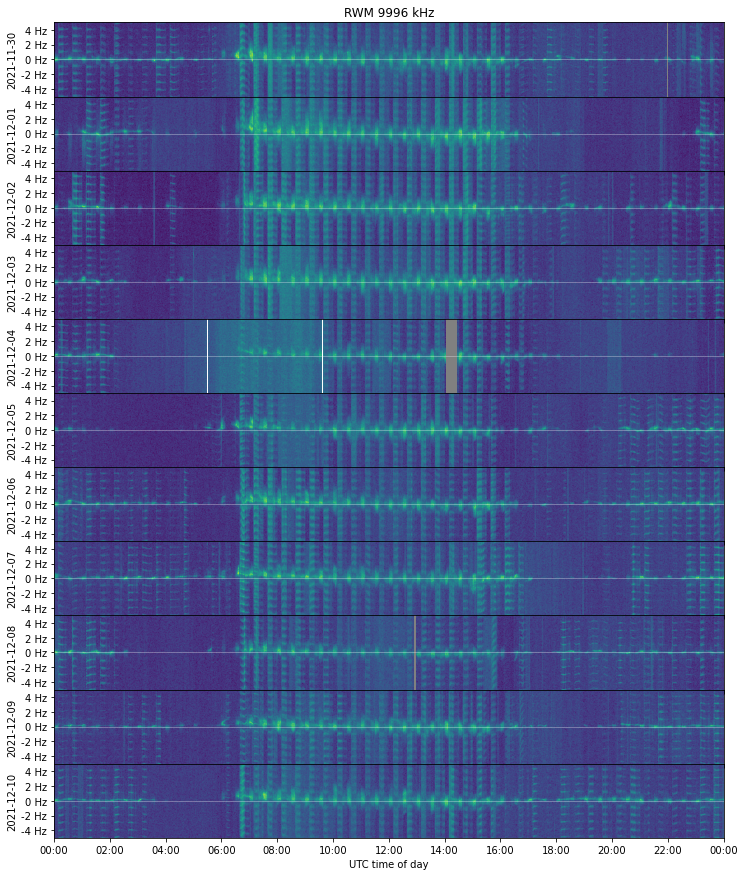
The first plot correspond to RWM at 4996 kHz. The plots for RWM don’t look good because the station only has a continuous carrier for 7 minutes 55 seconds starting at 0 and 30 minutes in the hour. The remaining time is spent sending either 1 Hz pulses or 10 Hz pulses, which cause sidebands in the spectrum.
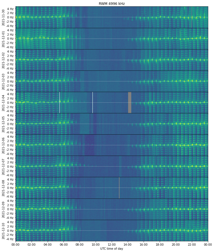
The 0 Hz reference has been marked with a faint white line to make easier to see the Doppler of the carrier. The start and end of the eclipse on December 4 have been marked with white vertical lines. There are some gray blocks in the waterfall that correspond to gaps in the data.
Additionally, the last segment of data, starting at 2021-12-08 12:57 UTC, should be taken with a grain of salt, because due to a problem (described in more detail in the Zenodo dataset) the Hermes-Lite 2 was using its internal TCXO rather than the external 10 MHz reference. I have corrected by hand the frequency offset of the TCXO, but there is still some frequency drift in the TCXO. This will be seen better in the plot corresponding to WWV at 10000 kHz.
We see that the propagation at 5 MHz is nocturnal. Additionally, in the morning we see a positive Doppler drift as the signal disappears, and in the evening we see a negative Doppler drift as the signal reappears. This makes sense because the virtual ionospheric layer height decreases at dawn, causing a positive Doppler shift, and increases at dusk, causing a negative Doppler shift.
The next plot shows WWV at 5000 kHz. This is the signal that has worked better for my station, because the signal is relatively strong and the continuous carrier makes much easier to see what is going on in contrast with RWM.
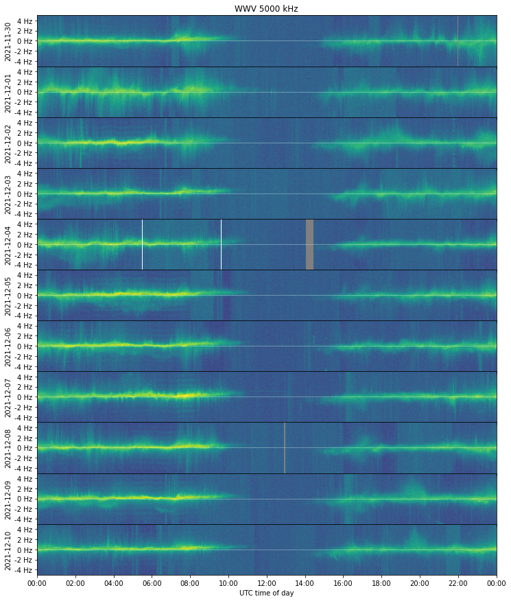
As in the case of RWM, propagation is nocturnal, and we also see the characteristic Doppler shifts in the morning and evening. I am amazed by how much richness there is in the data. Besides the Doppler frequency and signal power, we have the Doppler spread, which causes really complex and interesting patterns. We can see that not only the total spread is sometimes larger and sometimes smaller (and this is typically correlated with the signal strength), but also at times the spread is noticeably asymmetric. It is not so clear how to process this data to try to extract some characteristics of the Doppler spread, but I am thinking of an approach based on estimating the central moments of the power spectral density.
For RWM at 9996 kHz we see that the propagation is strong during daytime, while there is sometimes also a weaker propagation at night. On the morning, the daytime propagation at 9996 kHz starts more or less at the same time that the 4996 kHz signal disappears, and the same happens in reverse during the evening.
The results for WWV at 10000 kHz are bad because the 10 MHz reference from the GPSDO leaks in with noticeable power (it can be seen as a thin steady line here) and the signal from WWV is not particularly strong and has a lot of spread. I’m not even certain that I’m only receiving WWV, since there are several stations in the world using 10000 kHz.
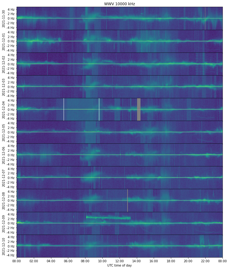
We can use this plot to assess the quality of the last segment of data, where the TCXO of the Hermes-Lite 2 was used instead of the GPSDO. Since we have the 10 MHz reference leaking in, any frequency drift we see in this reference is due to a drift in the TCXO. On December 8 the 10 MHz reference is very close to 0 Hz because I have corrected the frequency offset by hand. However, as time advances we can see the 10 MHz getting slightly higher in frequency. This is caused by the TCXO drifting down in frequency, probably due to ageing.
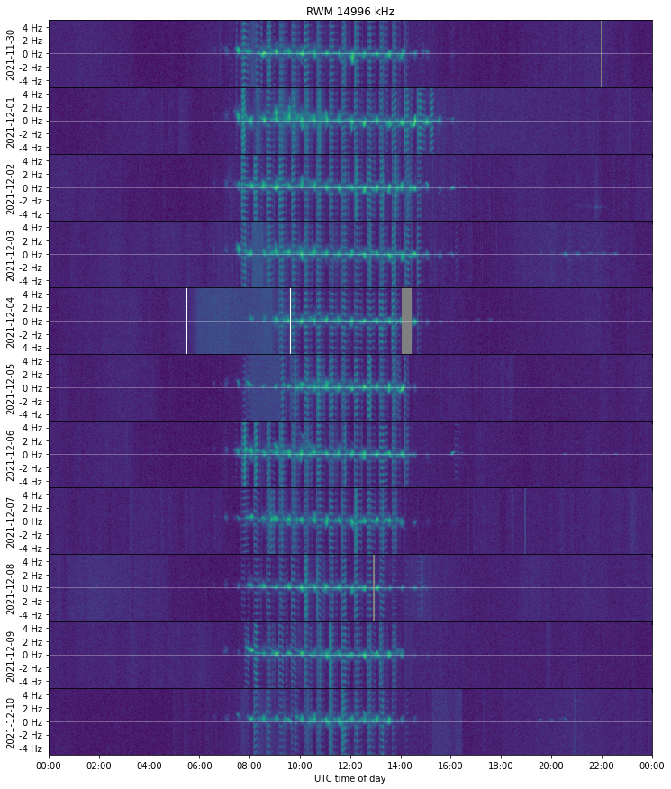
At 14996 kHz, RWM only shows diurnal propagation. In fact we see that the propagation in this band starts about 1 hour later than on 9996 kHz, and often ends 2 hours before. Also notice how the noise floor power has decreased in comparison with the lower frequency bands.
The recording of WWV at 15000 kHz is interesting because we see a signal between approximately 6:00 UTC and 9:00 UTC. Then we see a signal again between 14:00 and 18:00 UTC. The first signal stops abruptly, so that means that the transmitter shuts down at 9:00 UTC. I don’t think this first signal is WWV. It might be the Chinese BPM time signal, which also transmits at 15000 kHz. I haven’t found any source mentioning a time signal that shuts down at 9:00 UTC. The 200 Hz span used in the IQ recordings is too narrow to identify the stations (they often have time codes at 1 kHz offsets from the carrier), so I will need to conduct additional observations to identify the stations and also to verify that the signal we see at 5000 kHz is WWV rather than BPM.

I think that the second signal, which is visible between 14:00 and 18:00 UTC is indeed WWV, since this period corresponds to the time when the propagation path between WWV and my station (which is half of the USA and Canada and the North Atlantic) is in daytime.
Interesting that an increase in background noise during the eclipse is for most measurements quite visible. Wonder is this is more visible than the doppler effect?
Hi Victor, I think the increase in background noise is local interference and just a coincidence.
HI Daniel,
Two professional life-times ago, I was in optical radiation metrology, spending most of my time in visible transmission and reflection spectroscopy. Nearly all of my computing was done in APL to ease the statistical computations of my data. As a result, I am low on the learning curve dealing with compiled languages.
I am intrigued by your frequency measurements and would like to work on similar tasks with GNU Radio. Last year, I got a Hermes Lite 2.0 and have it working with my GPSDO using Thetis (checkbox in setup…no programming). I am stuck in a Windows 10 environment with no real options to change. The latest GNU Windows installation uses Python 3.9 and your blocks apparently don’t work with it (I haven’t tried).
If you could help me a little to figure out how to get GRC working in my environment, or point me in the right direction, I would be very appreciative. Thanks
Hi Davie,
I haven’t ported gr-hermeslite2 to GNU Radio 3.9. I might do that at some point, but even so it’s tricky to build out-of-tree modules in Windows. The easiest way of installing GNU Radio out-of-tree modules is perhaps through Conda, but that requires OOT module maintainers to create the Conda package. In this case gr-hermeslite2 is a module that few people use, so I’m not certain if it’s worth the effort. Perhaps you could try running GNU Radio in a Linux virtual machine. Since the Hermes-Lite 2.0 doesn’t stream a lot of bandwidth and runs on the network, I don’t think performance will be so much of a problem, as with other SDRs.
Thanks for the direction. I’ll look into it. Hoping to do some exciting work with it.
Dave (I misspelled my name before)