Decoding James Webb Space Telescope

The James Webb Space Telescope probably needs no introduction, since it is perhaps the most important and well-known mission of the last years. It was launched on Christmas day from Kourou, French Guiana, into a direct transfer orbit to the Sun-Earth L2 Lagrange point. JWST uses S-band at 2270.5 MHz to transmit telemetry. The science data will be transmitted in K-band at 25.9 GHz, with a rate of up to 28 Mbps.

After launch, the first groundstation to pick the S-band signal from JWST was the 10 m antenna from the Italian Space Agency in Malindi, Kenya. This groundstation commanded the telemetry rate to increase from 1 kbps to 4 kbps. After this, the spacecraft’s footprint continued moving to the east, and it was tracked for a few hours by the DSN in Canberra. One of the things that Canberra did was to increase the telemetry rate to 40 kbps, which apparently is the maximum to be used in the mission.

As JWST moved away from Earth, its footprint started moving west. After Canberra, the spacecraft was tracked by Madrid. Edgar Kaiser DF2MZ, Iban Cardona EB3FRN and other amateur observers in Europe received the S-band telemetry signal. When Iban started receiving the signal, it was again using 4 kbps, but some time after, Madrid switched it to 40 kbps.

At 00:50 UTC on December 26, the spacecraft made its first correction burn, which lasted an impressive 65 minutes. Edgar caught this manoeuvre in the Doppler track.

Later on, between 7:30 and 11:30 UTC, I have been receiving the signal with one of the 6.1 metre dishes at Allen Telescope Array. The telemetry rate was 40 kbps and the spacecraft was presumably in lock with Goldstone, though it didn’t appear in DSN now. I will publish the recording in Zenodo as usual, but since the files are rather large I will probably reduce the sample rate, so publishing the files will take some time.

In the rest of this post I give a description of the telemetry of JWST and do a first look at the telemetry data.

The lower rate configurations of the telemetry signal of JWST use PCM/PSK/PM with a 40 kHz subcarrier, while the 40 kbps configuration uses PCM/PM/NRZ. The spacecraft uses CCSDS concatenated coding, so the 4 kbps configuration actually corresponds to exactly 8 kbaud, while 40 kbps is 80 kbaud.

According to the data recorded by Iban, the 4 kbps telemetry uses a single (252, 220) Reed-Solomon codeword. This choice is interesting, because it gives a frame size of 2048 bits at the input of the convolutional encoder, taking into account the ASM. Several Chinese missions such as Tianwen-1 and Chang’e 5 have used this codeword size, because the baudrates they use are powers of two, such as 2048 or 16384 baud. By having 2048 bit frames, the get a nice round value for the time it takes to transmit a frame, such as 2 seconds, or 0.25 seconds. However, in the case of JWST the baudrate is not a power of 2, but rather a “nice round number in base 10”, such as 4000 or 40000. Therefore, they don’t get these nice round durations for the frames. Thus, it is curious that they have chosen the shortened size of (252, 220) rather than the full size of (255, 223).

The 40 kbps telemetry uses 5 interleaved (252, 220) Reed-Solomon codewords, so the total frame size is 1100 information bytes.

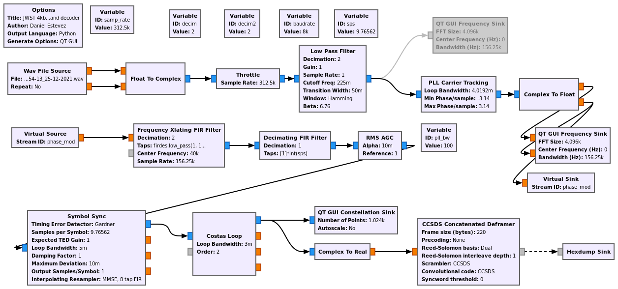
The GNU Radio decoder flowgraph that I used with Iban’s recording, which contains 4 kbps telemetry, can be downloaded here. It is shown in the figure below.

Unfortunately, the SNR in Iban’s recordings is slightly less than needed for decoding, and I haven’t been able to get a single Reed-Solomon frame decoded correctly. Still, taking into account that the data has errors, one can look at the frames and learn some things, since the Reed-Solomon code is systematic. This is what r00t.cz has been doing with the recordings.

For the 40 kbps telemetry in the ATA recordings I have used this flowgraph, which is shown here.

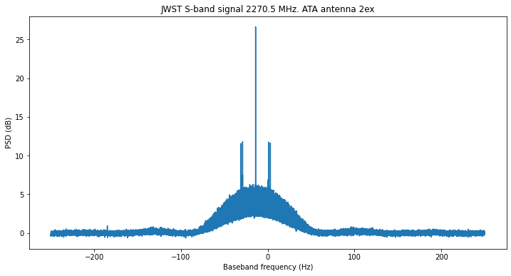
The antenna feeds in the ATA use dual linear polarization (X and Y), so the Auto-polarization block combines the two polarizations to maximize the SNR. The signal from JWST is nominally circularly polarized (RHCP, I think), but since the low gain antenna is a patch antenna and we don’t see it directly from its boresight direction, in general we will see some elliptical polarization (see my post about the Chang’e 5 polarization). I observed that at the beginning of the recording there was much more signal power in the X polarization than in the Y polarization. I will have to check how this evolves throughout the recording. The figure below shows the spectrum of the signal using only the X polarization.

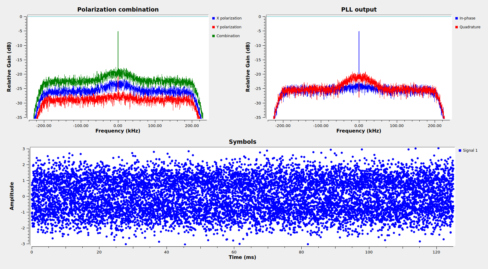
The SNR in the X polarization is barely enough to decode, and some of the frames can be decoded, but others not. By combining both polarizations we gain some SNR and it is possible to decode a large fraction of the frames.

The figure below shows the GUI of the GNU Radio decoder running with the beginning of the ATA recording. We can see the difference of SNRs between the X and Y polarizations in the upper left spectrum plot. We see that the symbols are very noisy, so it almost seems magic that the Viterbi and Reed-Solomon decoder are able to decode so many correct frames.

The frames transmitted by JWST are CCSDS AOS frames. The spacecraft ID is 170 (0xaa), which matches the ID used in NASA HORIZONS and the SANA registry. There are two virtual channels in use, virtual channel 0, which carries the telemetry, and virtual channel 63, which is Only Idle Data. The Only Idle Data frames have all the payload (everything besides the AOS primary header) filled with 0x78 bytes, which is ASCII for x.

Approximately 95% of the frames belong to virtual channel 0. The frames in virtual channel 0 contain CCSDS Space Packets using the M_PDU protocol. The last 4 bytes of the frame are a trailer. It seems that the contents of the trailer cycle through the values 0x010001eb, 0x0904019e, and 0x09080100 every three frames (at least near the beginning of the recording). I am not sure what this trailer represents. I don’t think it is a Communications Link Control Word (as described in the CCSDS TC Space Data Link Protocol) because one of the reserved bits is set to one instead of zero as it should. However I can’t rule out the possibility completely, since the values of the rest of the fields could make sense.

The figure below shows the number of frames lost in virtual channel 0 according to the jumps in the virtual channel frame counter. We can see that towards the end of the recording, as the spacecraft elevation decreases and eventually goes under the elevation mask, the error rate increases. Overall, 76% of the frames in virtual channel 0 have been decoded correctly.

Many Space Packet APIDs are active. As usual, I have done raster plots of each of them in a Jupyter notebook. Glancing through these raster plots, my impression is that there are many that have complex data structures, though there are also many zones padded with zeros. The two figures below show some examples of how the APIDs look like. The full list of plots can be seen in the Jupyter notebook.

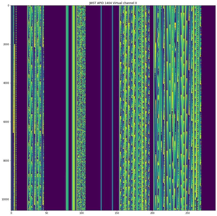
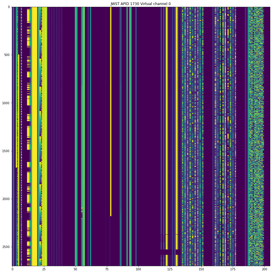
I have also seen that there are many fields with floating point numbers. These usually have a distinct “texture”, so they are not so difficult to spot in these raster plots.

I have tried to go through all the APIDs, plotting the values of all the floating point fields, though I haven’t tried to be exhaustive and might have left some. I haven’t seen any that look as interesting as the state vector data of Tianwen-1. Most of the floating point fields are 32-bit wide (using IEEE 754 big-endian representation), but there are a few that are 64-bit wide.

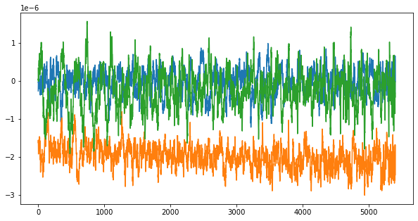
Perhaps the floating point channels that I have found more interesting are these adjacent three, which appear in APID 1201, and also in APIDs 1404 and 1727 (in several cases it seems that the same or very similar data appears in some fields of several different APIDs).

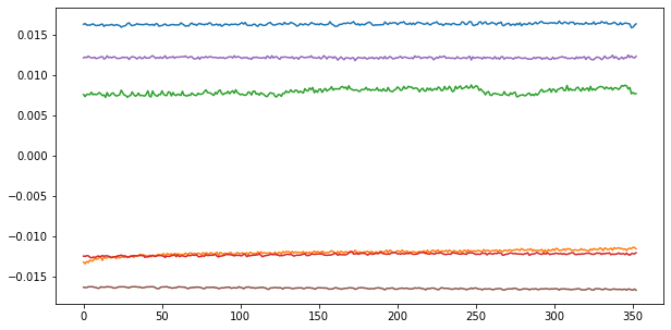
Another set of floating point channels which looks interesting are the following 6 adjacent channels in APID 1755.

The full list of these plots is also in the Jupyter notebook. At the moment I have no idea of what kind of data any of them are showing. One should be careful when interpreting the data, because there is even the chance that some of the fields are not really floating point, but integers, even though they have reasonable values when interpreted as floating point.

Probably I’ll come back to these recordings in the next few days, but for now I wanted to publish what I have so far. The decoded frames are available in the Github repository and can be obtained using git-annex as described in the README.