radar – Daniel Estévez

Analysis of the CAMRAS Venus radar experiment

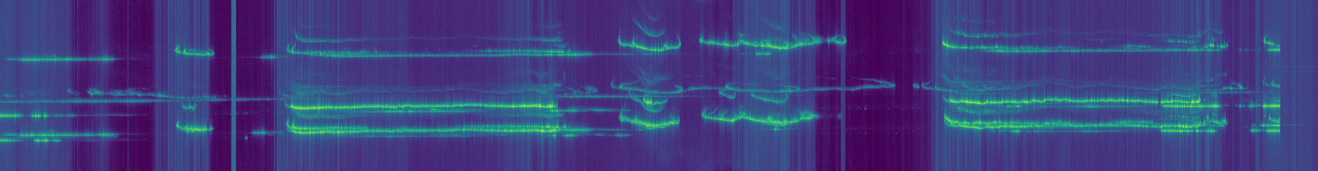
On March 22, CAMRAS performed a Venus radar experiment (or Earth-Venus-Earth bounce, as it is more commonly known in Amateur radio) in collaboration with Astropeiler Stockert, the Deep Space Exploration Society, and the Open Research Institute. The experiment was done in L-band, at 1299.5 MHz, using the 25 m Dwingeloo radiotelescope as transmitter and receiver and the Stockert 25 m telescope as a receiver. The experiment was done during the Venus conjunction, as this minimizes the distance between the Earth and Venus. The round-trip time to Venus was approximately 280 seconds. The radar waveform was a CW carrier with a duration of 278 seconds. It was transmitted a total of 4 times every 600 seconds. Thus each period was composed by:

278 second transmission
~2 second TX/RX guard time
278 second echo reception
~42 second wait

More transmissions were planned, including some spread-spectrum signals designed by the Open Research Institute. However, the transmitter started failing and they had to stop.

Update 2025-04-21: I have been informed that the spread-spectrum signal for this experiment was designed by CAMRAS. The waveform that the Open Research Institute is designing will potentially be used in future experiments.

CAMRAS has published an analysis of the recorded IQ data, showing successful echo detections with Dwingeloo and Stockert. There is an example Jupyter notebook that shows how to Doppler correct the echo and detect it with an FFT. All the recorded IQ data has been published.

In this post I will do my own analysis of the experiment. The goal is not to confirm the successful detection with an independent analysis, since I believe that the analysis published by CAMRAS is correct and leaves no doubt about this. It is to expand this analysis and to touch on other topics that this analysis has not covered:

Calculation of the Doppler. CAMRAS has published CSV files containing the expected Doppler at each receiver, but they have not published the code to calculate this. Here I will do all the relevant calculations with SPICE.
Doppler correction with the gr-satellites Doppler correction block, which performs linear interpolation of the Doppler frequency to calculate the frequency shift applied to each sample.
High-quality spectral analysis with a polyphase filterbank.
Try to estimate the Doppler spread and compare with some results in the literature.

Lunar reflections during SLIM landing

In my previous post, I looked at the Doppler of the SLIM S-band telemetry signal during its landing on the Moon. I showed some waterfall plots of the signal around the residual carrier. In these, a reflection on the lunar surface was visible. The following figure shows a waterfall of the signal around the residual carrier, after performing Doppler correction and using a PLL to lock to the residual carrier. I was intrigued by the patterns made by these reflections, specially by some bands that look like a ‘1’ shape (the most prominent happens at 14:58).

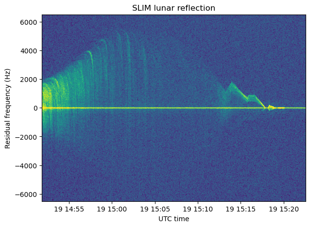
In this post I study the geometry of the lunar reflection and find what causes these bands.

BPSK pulse radar revisited

Some months ago I published the analysis of a BPSK pulse radar waveform that Scott Tilley VE7TIL had received through the transponder of Meridian 8 at a downlink frequency of 994 MHz. Now Roland Proesch DF3LZ has analyzed the same recording that I used, finding some different signal parameters. This has made me review my analysis, and it turns out that I made a mistake in finding the symbol rate of the signal. This post is an updated analysis, correcting my mistake.

BPSK radar received through Meridian 8

Ever since SETI Insitute published the news of a possible signal received from Proxima Centauri in some of the Parkes telescope recordings at 982 MHz, Scott Tilley VE7TIL has taken up the interest to search and catalogue the satellites that transmit on this band (specially old, forgotten and zombie satellites). His idea is to try to see if this candidate signal can be explained as interference from some satellite.

This has led him to discover some signals coming from satellites on a Molniya orbit. After examination with the Allen Telescope Array of these signals, we confirmed that they came from wideband transponders (centre frequency around 995 MHz, 13 MHz width) on some of the Meridian Russian communications satellites (in particular Meridian 4 and 8, but also others).

These transponders show all sorts of terrestrial signals that are relayed as unintended traffic through the transponder. By measuring Doppler we know that the uplink is somewhere around 700 or 800 MHz. We have found some OFDM-like signals that seem to be NB-IoT. Unfortunately we haven’t been able to do anything useful with them, maybe because there are several signals overlapping on the same frequency. We also found a wideband FM signal containing music and announcements in Turkmen, which later turned out to be the audio subcarrier of a SECAM analogue TV channel from Turkmenistan.

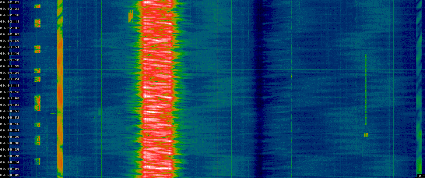
A few days ago, Scott detected a pulsed strong signal through the transponder of the Meridians at a downlink frequency of 994.2 MHz. He did an IQ recording of this signal on the downlink of Meridian 8. It turns out that this signal is a BPSK pulse radar. In this post I do a detailed analysis of the radar waveform using this recording.

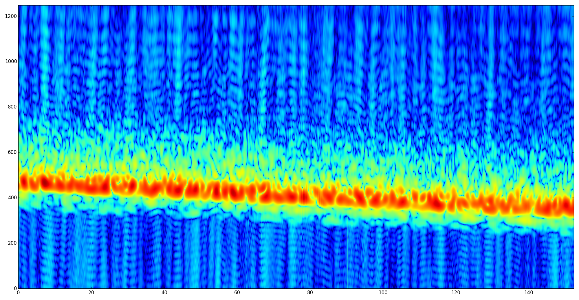
Using CODAR for ionospheric sounding

CODAR is an HF radar used to measure surface ocean currents in coastal areas. Usually, it consists of a chirp which repeats every second. The chirp rate is usually on the order of 10kHz/s, and the signal is gated in small pulses so that the CODAR receiver can listen between pulses. The gating frequency can be on the order of 1kHz.

CODAR can be received by skywave many kilometers inland. Being a chirped signal, it is easy to extract the multipath information from the received signal. In this way, one can see the signal bouncing off the different layers of the ionosphere, and magnificent pictures showing the changes in the ionosphere (especially at dawn and dusk) can be obtained. For instance, see these images by Pieter Ibelings N4IP, or the image at the top of this post, which contains 48 hours worth of CODAR data.

Here I describe my approach to receiving CODAR. It uses GNU Radio for most of the signal processing, and Python with NumPy, SciPy and Matplotlib for plotting.

Improving signal processing in my OTH radar receiver

This is a follow up post to my experiments studying OTH radar. I have found that the signal processing I did there to obtain the cross-correlation was far from optimal. This produced the strange side-bands below the main reflection. The keen reader might have noticed that I was doing the cross-correlation with a template pulse that lasted the whole pulse repetition cycle. However, the pulses from the radar are shorter. Therefore, it is a better idea to use a shorter template pulse. Ideally, the template pulse should have the same length as the transmitted pulse. However, I don’t know this length precisely, because multipath propagation makes the received pulses a bit longer. However, I think that 6.5ms is a good estimate.

I have also changed the window for the pulse. I’m now using a Dolph-Chebyshev window. I use scipy to compute this window, because it is not included in GNU Radio. This window has the property that the side-bands have constant attenuation. Indeed, it minimizes the \(L^\infty\) norm of the side-bands. There is a parameter that tunes the side-bands attenuation. For higher attenuations, you have a wider main lobe, while if you want a narrower main love you get less side-band attenuation. These properties make this window useful in radar applications.

Below I’m doing the cross-correlation in GNU Radio with a shorter template pulse shaped with a Dolph-Chebyshev window set for 55dB attenuation.

The good thing about the settable attenuation of the Dolph-Chebyshev window is that it can be used to trade-off performance between different features. First, we use an attenuation of 100dB. The side-bands are below the noise floor in this case, so we have no “false responses” in our cross-correlation. The drawback is that the main lobe is wide so the resolution of the features of the ionosphere in the image below is not very good.

Dolph-Chebyshev window with 100dB attenuation

Next we try with 55dB attenuation. This narrows the main lobe, improving the resolution and crispness of the features of the ionosphere in the image below. However, side-bands start being visible above the noise floor, producing “false responses”. However, comparing with the image above, we now know where the false responses are.

Dolph-Chebyshev window with 55dB attenuation

I have updated the gist with the GNU Radio flowgraph and python script used to produce the images.

Looking at an HF OTH radar

Most amateur operators are familiar with over-the-horizon radars in the HF bands. They sometimes pop up in the Amateur bands, rendering several tens of kilohertzs unusable. Inspired by Balint Seeber’s talk in GRCon16, I’ve decided to learn more about radars. Here I look at a typical OTH radar, presumably of Russian origin. It was recorded at my station around 20:00UTC on 8 December at a frequency around 6860kHz. This radar sometimes appears inside the 40m Amateur band as well.