Ever since SETI Insitute published the news of a possible signal received from Proxima Centauri in some of the Parkes telescope recordings at 982 MHz, Scott Tilley VE7TIL has taken up the interest to search and catalogue the satellites that transmit on this band (specially old, forgotten and zombie satellites). His idea is to try to see if this candidate signal can be explained as interference from some satellite.
This has led him to discover some signals coming from satellites on a Molniya orbit. After examination with the Allen Telescope Array of these signals, we confirmed that they came from wideband transponders (centre frequency around 995 MHz, 13 MHz width) on some of the Meridian Russian communications satellites (in particular Meridian 4 and 8, but also others).
These transponders show all sorts of terrestrial signals that are relayed as unintended traffic through the transponder. By measuring Doppler we know that the uplink is somewhere around 700 or 800 MHz. We have found some OFDM-like signals that seem to be NB-IoT. Unfortunately we haven’t been able to do anything useful with them, maybe because there are several signals overlapping on the same frequency. We also found a wideband FM signal containing music and announcements in Turkmen, which later turned out to be the audio subcarrier of a SECAM analogue TV channel from Turkmenistan.
A few days ago, Scott detected a pulsed strong signal through the transponder of the Meridians at a downlink frequency of 994.2 MHz. He did an IQ recording of this signal on the downlink of Meridian 8. It turns out that this signal is a BPSK pulse radar. In this post I do a detailed analysis of the radar waveform using this recording.
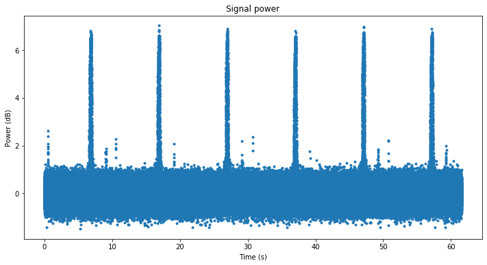
As a first step, the meridian_pwr.grc GNU Radio flowgraph is used to compute average power in windows of 100 us. The results of this are plotted below. The figure shows strong pulses appearing every 10 seconds approximately.
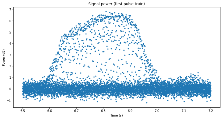
If we zoom in to any of these pulse we see that in fact it consists of a train of very short pulses. At a 100 us resolution, the pulses only last two time bins.
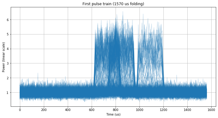
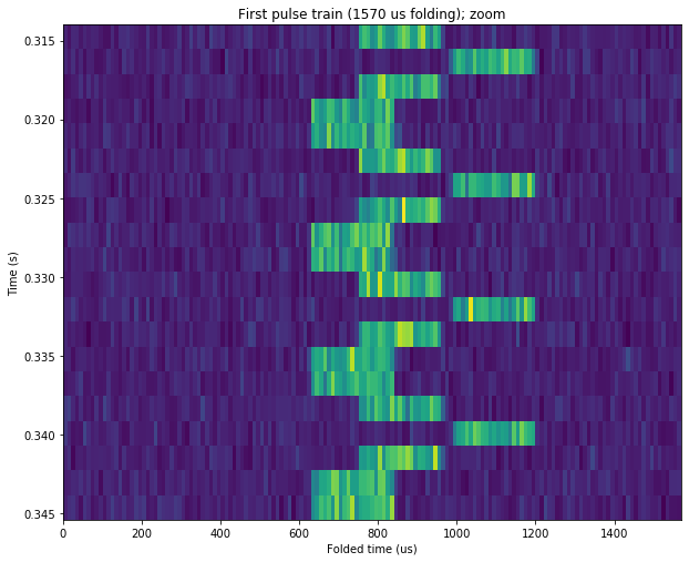
To obtain more resolution, it is appropriate to work directly with the IQ data. Since the full one minute recording is large, we work only with the first pulse train. After some careful analysis, it turns out that the pulses can be folded neatly by using a period of exactly 1570 us. However, when folding by 1570 us we see that the pulses actually happen at three different positions.
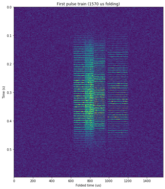
This is called pulse staggering and it is pretty common in radar. The figure below shows the staggering more clearly. Here each line represents a 1570 us period. We can see the three different pulse positions, which follow a very regular pattern. It is also noteworthy how the pulse train fades in and out.
Zooming in to one small piece of this image we see more clearly the pulse staggering pattern. The offsets of the pulses follow the repeating sequence [0, 1/2, 3/2, 1/2, 0], where here one unit is approximately equal to the pulse length.
Next we analyse one of these pulses separately. If we compute the square of the signal we see that its spectrum has a strong CW tone. This suggests that the pulse is BPSK-modulated. The frequency of the tone allows us to recover the suppressed carrier, which is at approximately -91.7 kHz in the 2Msps IQ recording. The cyclic autocorrelation function has a cycle frequency at nearly 800 kHz, which indicates that the baudrate is 800 kbaud. Using this data we can perform carrier and clock recovery manually and obtain the BPSK symbols. The image below is the final result, and shows the BPSK symbols in the I component, and noise in the Q component.
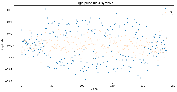
The BPSK constellation is a bit noisy, because the pulse doesn’t have a large Es/N0 (it’s around 10dB), and it is not so easy to tell exactly when the pulse starts and ends. To increase the SNR of the BPSK symbols, we can check whether all the pulses use the same sequence of symbols (this will most likely be the case for a radar waveform) and accumulate all the pulses coherently.
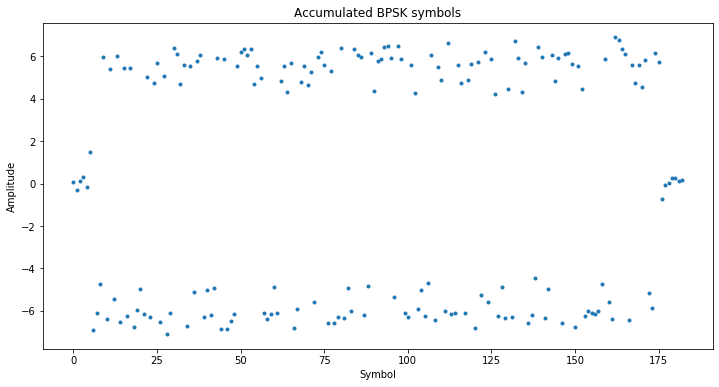
In order to perform this accumulation, the first pulse train is folded in 1570 us segments, and one of the folds that contains a stronger pulse is chosen as a reference (the 100th fold, actually). All the folds are correlated against the reference fold and then cyclically shifted to align them in time with the reference and multiplied by a complex phasor to align them in phase. Then all the folds are summed coherently. The result is shown below. We can see a strong BPSK pulse in the I component, and some of the BPSK signal leaking into the Q component because the phase alignment wasn’t perfect.

If we zoom in to the BPSK pulse, we clearly see the BPSK waveform

Clock recovery is performed again manually, obtaining the symbols below, where now it is very clear where the pulse starts and ends.
The symbol sequence can now be extracted without errors. The length of the sequence is 170 bits and its contents are shown below. Note that we have a 180º phase ambiguity that we are not able to solve, so it is quite possible that the waveform designers considered the same sequence but swapping the 0’s and 1’s.
000101010101000010110100111101011000010100011111111000001
111001111011101001000111001111111011001100001011010011011
01010110001011110001100111011101100000010011110111110011
As a consistency check, and to show that all the pulses indeed have the same sequence, I checked that the sequence decoded from the single pulse shown above coincides with this sequence exactly (so in fact we were able to demodulate the single pulse without bit errors).
The autocorrelation of this 170 bit sequence is shown here. It is noteworthy that the sidelobes near the main peak are very small. Random sequences usually have worse sidelobes than this, so I think that this is a sequence optimized for this property.
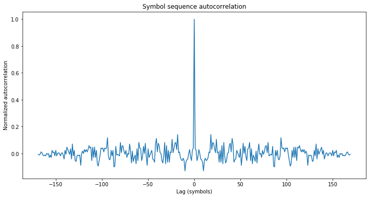
Small sidelobes near the main peak are an important property for radar because the sidelobes decrease the resolution for estimating the target range, and for discerning separate targets at similar ranges. Constructing long sequences with small sidelobes mathematically is a difficult problem (see Barker codes), so these sequences are usually found by search and optimization methods.
A quick and easy method to build sequences having good autocorrelation properties is to use maximum length sequences. These are optimal for circular autocorrelation, but not so good for linear autocorrelation, which is the important property for pulse radar. Maximum length sequences have several interesting properties. One of them is that a maximum length sequence of length \(2^n – 1\) contains, as subsequences of length \(n\), all the possible \(n\)-bit subsequences except for the sequence that consists of all zeros. Moreover, each of these \(n\)-bit subsequences appears exactly once. (One should consider the maximum length sequence cyclically when taking all its possible \(2^n-1\) subsequences of length \(n\)).
Using this property it is easy to check if a given sequence can be a subsequence of a maximum length sequence of length \(2^n -1\), just by checking if there are some two subsequences of length \(n\) that are equal. The 170 bit sequence of this radar has two 15 bit subsequences that are equal, so it can’t be a subsequence of a maximum length sequence of length \(2^n – 1\) with \(n <= 15\). This doesn’t preclude the possibility that the 170 bit sequence is a subsequence of a maximum length sequence with larger \(n\) (and in fact it will always be a subsequence of maximum length sequences with \(n >= 170\)), but it wouldn’t make sense to design a 170 bit sequence by taking a small subsequence of a large maximum length sequence.
Now that we have extracted the 170 bit sequence and the baudrate, we can generate the pulse waveform in GNU Radio and correlate it against the IQ recording. Since the correlation of the recording would be large (having the same length as the recording) but we are only interested in the correlation peaks produced by pulses, I have made a Python block that produces a sparse signal. This block only outputs signal samples whose amplitude exceeds a certain threshold, together with their position on the sample stream. In this way, the output file is very small, but the pulse position, amplitude and phase is preserved exactly. The GNU Radio flowgraph that uses this technique is called meridian_corr.grc.
The figure below shows the amplitude of the correlation with the pulse waveform, as obtained from the sparse representation of the GNU Radio flowgraph output. We see something very similar to the figure at the beginning of the post, with pulse trains every 10 seconds or so.

The correlation peaks of the pulses span 5 samples, since the signal is sampled at 2.5 samples per symbol. Therefore, we use a peak find algorithm to extract only the peak of each of the pulses. An easy improvement of this algorithm would use interpolation to find the peak position more accurately, since it will typically lie somewhere between two consecutive samples. In the sequel, we work only with the pulse peaks.
The periodicity of the pulse trains corresponds to the sweep period of the radar. It is very likely that this radar sweeps a a narrow beam scanning 360 degrees of azimuth every 10 seconds, and only when the radar beam points towards the satellite (which is most likely near the horizon, as it happens with the Turkmen TV station) we see the radar pulses.
We can measure the sweep period more carefully, and it turns out to be 10.07 seconds. When we fold the plot with this period, all the sweeps lie neatly on top of each other, as shown here.
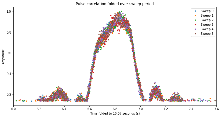
This figure shows other interesting aspects regarding the amplitude profile of the sweep. We can see some sidelobes, which would correspond to sidelobes of the radar beam. The asymmetry of the main lobe is also interesting. I don’t know why this happens.
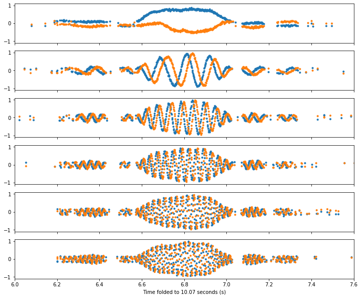
The figure below shows the I (blue) and Q (orange) components of the pulse peaks. The IQ recording has been shifted in frequency to move the pulses to baseband using the frequency of the first sweep. As Doppler changes, the subsequent pulses show higher and higher frequency.
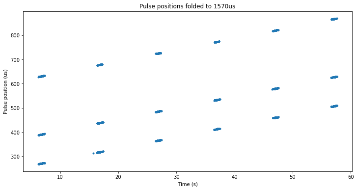
Next we study the pulse positions in detail. The figure below shows the pulse positions folded to the 1570 us repetition rate. We see three lines corresponding to the pulse staggering. The lines slope up with time because of the change in two-way range between the transmitter and receiver, and their relative clock drifts.
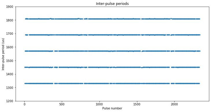
To study the staggering, we subtract the pulse positions of adjacent pulses to obtain the inter-pulse periods. We see that there are five different inter-pulse periods. These are 1330, 1450, 1570, 1690, and 1810 us. They correspond to a pulse staggering pattern of 0, 120, 360, 120, and 0 us. Above we said that the staggering pattern was, in some arbitrary units of size close to the pulse length, 0, 1/2, 3/2, 1/2, 0, so we see that one unit corresponds to 240 us. In comparison, a 170 bit pulse at 800 kbaud has a length of 212.5 us.
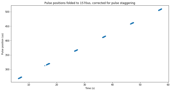
After correcting the folded pulse positions for pulse staggering, we obtain the figure below, where all the pulses are now neatly aligned.
The rate at which the pulse positions drift corresponds to a speed of 1409 m/s. At the time that the recording was made, Meridian 8 had a range rate of 336 m/s with respect to Scott’s station. Since the satellite was near its Molniya orbit apogee, the range rate as seen from other groundstations in the footprint would be similar to this, around 300 or 400 m/s.
Thus, I believe that a good amount of this 1409 m/s drift rate is due to the transmitter and receiver clock offsets. I’m not sure if Scott was using a GPSDO reference for this recording, but probably the radar isn’t, as there is no need to clock very precisely a monostatic radar. The drift rate is 4.7 ppm, so this clock error is quite reasonable for a transmitter that isn’t locked to GPS. Therefore, I don’t think it’s possible to use the drift rate information to say anything about the transmitter location, because the range rate and the clock drift get mixed up in the observation equation (there is only one equation and two unknowns).
The plots and calculations in this post were done in this Jupyter notebook, which contains some additional figures. The repository also contains the GNU Radio flowgraphs and the data, except for the large IQ recording.
The recovery of the 170 bit BPSK sequence was loosely inspired by a write up from the people of the Cornell University GPS laboratory about the determination of the GIOVE PRN codes.
Nice work, once again!
Nice work