Some months ago I published the analysis of a BPSK pulse radar waveform that Scott Tilley VE7TIL had received through the transponder of Meridian 8 at a downlink frequency of 994 MHz. Now Roland Proesch DF3LZ has analyzed the same recording that I used, finding some different signal parameters. This has made me review my analysis, and it turns out that I made a mistake in finding the symbol rate of the signal. This post is an updated analysis, correcting my mistake.
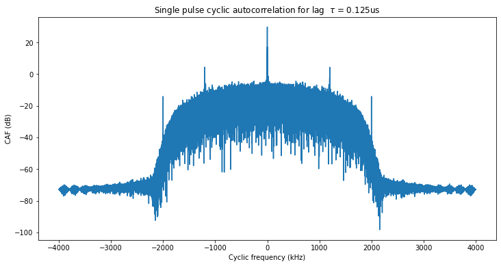
In my original analysis, I stated that the pulses of this radar were modulated with an 800 kbaud BPSK sequence of 170 symbols. As Roland found later, the symbol rate is actually 1.2 Mbaud. My mistake came because the recording is sampled at 2 Msps, so when working at 2 Msps IQ sampling, the 1.2 Mbaud symbol rate aliases down to 800 kbaud (for instance, when working with cyclostationary analysis).
Usually, a mistake like this caused by not noticing aliasing will be obvious, because attempting to recover the symbol clock with the wrong symbol rate will fail. There will be sampling points that lie halfway between two symbols, and this will be clear when plotting the constellation and the symbol amplitude versus time. However, in this case I was able to get a seemingly good symbol recovery, and so I proceeded forward inadvertently.
The reason why I got a seemingly good symbol recovery with the wrong symbol rate is quite interesting. First, note that by trying to interpret a 1.2 Mbaud waveform as 800 kbaud, the symbols we’re trying to use are actually 1.5 symbols long. This means that we can align our local clock in such a way that each of our sampling points is at a distance of 0.25 symbols from each of the actual symbols of the waveform. This happens just because of the unfortunately coincidence that we’re using a symbol period that is 1.5 symbols long, which ultimately comes from the unfortunate relation between the symbol rate and the recording sample rate. If our symbol clock was wrong by another factor, like say if it was 1.4 symbols long, then the error would accumulate as some sort of vernier scale, and the distance between the sampling points and the actual symbol locations will keep changing between 0 and 0.5 symbols as we move through the burst.
To make things worse, since I was lazy, instead of interpolating the samples to the required sampling points, I was just taking the nearest sample. Since a sample is 0.6 symbols long and we’re off by 0.25 samples, we’re always taking the sample that is closest to the actual symbol location. So in the end, we unknowingly skip one third of the symbols, but the symbols that we do take look perfect in the amplitude versus time and constellation plots.
To prevent this from happening, and also to get improved alignment when accumulating pulses from the same burst to increase the SNR, I have upsampled the recording by a factor of 4. The cyclostationary analysis now clearly shows the 1.2 Mbaud symbol rate, as indicated in the figure below.
Next we show the result of aligning and accumulating coherently all the pulses in a sweep. The BPSK sequence can be seen with high SNR and the symbol recovery, indicated by the orange dots is good.
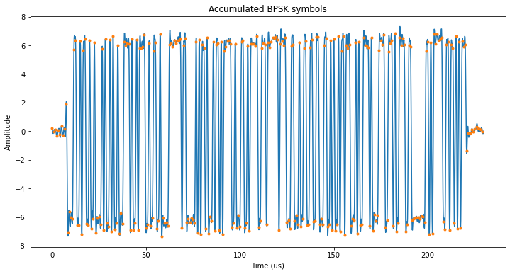
The length of the BPSK sequence is 255 symbols, which gives a pulse duration of 212.5 microseconds. This is the same that I had calculated in my previous post. The sequence is as follows:
0000110010110010010000101001010010001111010010111100100110
0100000111111110110000001010110100010110101111100100011001
0111110011101111111011110001100010011001100110001100101001
0110111000101001111010000111100111010011110011000000000110
10111111001101101010111
The length of 255 bits is quite typical, because it is the length of an m-sequence generated by an 8 bit LFSR. The linear and circular autocorrelations of this sequence are shown here.
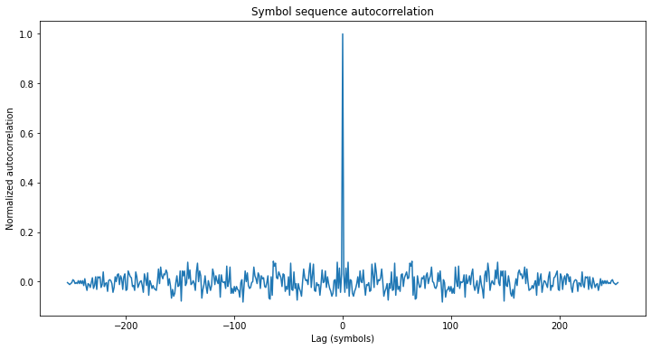

From the circular autocorrelation it is apparent that this sequence is not an m-sequence, because m-sequences have a normalized off-peak autocorrelation of -1/N, where N is the length of the sequence. Moreover, it seems that that the off-peak autocorrelation of this sequence is too large for it to be an optimized sequence, such as a Gold or Kasami code or a memory code. For instance, the standard deviation of the (not normalized) off-peak autocorrelation is 12.7, which is close to the square root of 255 (which is almost 16). Random sequences tend to have an off-peak autocorrelation around this value.
So it may well happen that this 255 bit sequence is cryptographically generated. This makes a lot of sense for a military radar. In order to make detection and spoofing more difficult, the sequence might be generated with a cryptographic key that keeps changing. In this case we see the same sequence being used throughout all the recording, but the recording is only one minute long, and key renewal periods will typically be longer than this. It would be interesting to search for this radar signal in a recording done on another day, to see if the sequence has changed.
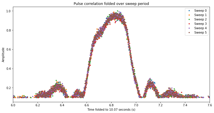
I have re-run the correlation with the new template pulse, also upsampling the recording by a factor of 4 to get better alignment. This has improved the plot shown below, which represents the amplitude of the correlation in each sweep. The time axis is folded to the sweep period of 10.07 seconds so that all the sweeps line up. Now we see that the amplitude pattern, which shows the beam gain pattern as the beam sweeps by the satellite, is perfectly repeatable between different sweeps, since the geometry hasn’t changed significantly over the course of one minute.
The remaining aspects of my analysis are unaffected by this correction about the symbol rate. I have updated my Jupyter notebook, GNU Radio flowgraph and related data files with this correction.