SLIM, JAXA’s Smart Lander for Investigating Moon, landed near Shioli crater on January 19. Shortly after the landing, the spacecraft was powered down to conserve power, since the probe had landed in an unexpected attitude which shaded its solar panels. After a few days of trying to contact SLIM, JAXA succeeded to reestablish communication with it on January 29. By then the Sun had moved west in the sky at SLIM’s location and had started illuminating the solar panels.
AMSAT-DL recorded the S-band signal from SLIM during the landing with the 20-meter antenna in Bochum Observatory. In this post I will analyse a recording done between 14:51:51 and 15:21:54 UTC (the touchdown was at 15:20 UTC). I will study the Doppler of the residual carrier and other radiometric quantities rather than the telemetry.
SLIM is transmitting a signal throughout all the recording, except for 2 seconds shortly after landing, when the transmitter turns off and turns on again. The spacecraft is in ground lock all the time, and an idle 2 kbps telecommand signal with a 16 kHz subcarrier is visible in the transponder.
The first step in the analysis is Doppler correction. HORIZONS has data for SLIM, but it says “Post-launch trajectory from JAXA. Data through January 18, prediction thereafter.” The relevant file is
 File name                                        Begins (TDB)     Ends  (TDB)
 ---------------------------------------------- -----------------  -----------
 20240119175154.202401190000.2024020100.burn.v1 2024-Jan-19 00:00  2024-Jan-31
I haven’t found any publicly available SPICE kernels.
After some attempts at Doppler correction, I realized that SLIM was in coherent Doppler mode with a groundstation in Japan transmitting at a constant uplink frequency. I haven’t found any official confirmation for the location of SLIM’s grounstation. There is some word in Twitter that it is Chiba, but for simplicity I have used Usuda, since the location of the deep space antenna is already in HORIZONS. There is not much difference, since Usuda is only 1.8 degrees west of Chiba.
To generate the Doppler files required by the Doppler correction GNU Radio block, I have used a script that I prepared for last year’s BSRC REU GNU Radio tutorials. This fetches the data from HORIZONS using Astroquery and writes the Doppler file in the required format. I have run the script as follows to generate the Doppler files for Bochum and Usuda. Due to the frequency multiplication done by the spacecraft transponder, the Doppler correction needs to be done using the downlink frequency, around 2212 MHz, for both the uplink and downlink legs of the path.
./horizons_doppler_correction.py --carrier-frequency 2212 \
    --observatory Bochum --spacecraft SLIM \
    --start-epoch 2024-01-19T14:30:00 --duration 3600 \
    --time-step 1 \
    --output-file SLIM-doppler-Bochum-2024-01-19.txt

./horizons_doppler_correction.py --carrier-frequency 2212 \
    --observatory Usuda --spacecraft SLIM \
    --start-epoch 2024-01-19T14:30:00 --duration 3600 \
    --time-step 1 \
    --output-file SLIM-doppler-Usuda-2024-01-19.txt
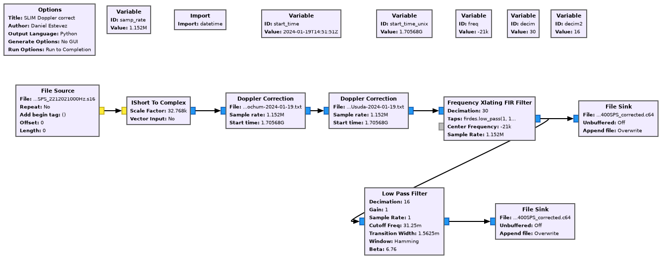
I have used this GNU Radio flowgraph to perform Doppler correction using two Doppler correction blocks and decimation. There are two output files. One at 38400 sps that is good to see the telecommand subcarrier and reflections of the residual carrier on the Moon (which can be up to 5 kHz away from the residual carrier), and one at 2400 sps, which is good to see the residual carrier in detail.
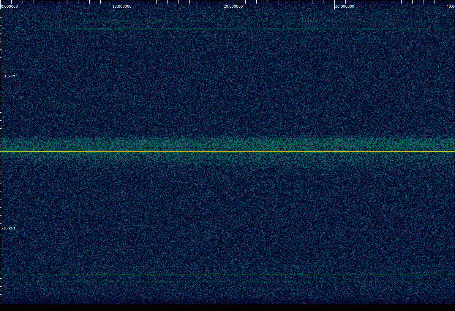
Here is how the waterfall of the beginning of the 38400 sps file looks like. We can see the residual carrier with a broad lunar reflection that spreads from -1 kHz to 2 kHz, and the idle telecommand subcarrier.
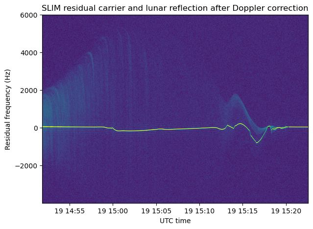
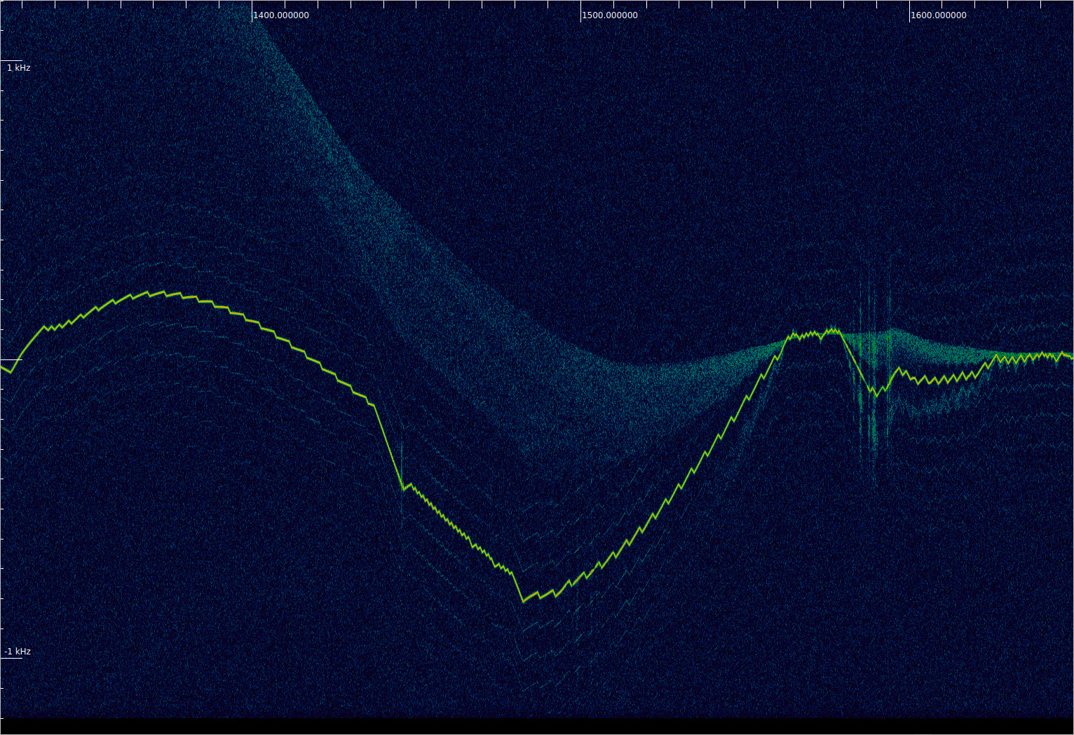
The reflection of the residual carrier on the lunar surface is best seen in the following waterfall, made with the full 38400 sps recording, and only showing the frequency range where the reflection appears. The patterns formed by the reflection look fascinating.
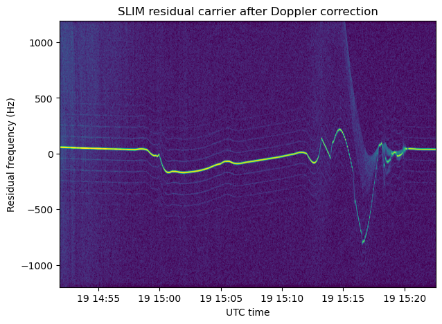
The next waterfall, obtained with the 2400 sps file, shows the residual carrier. All the frequency changes that we see here correspond to velocity changes that are not modelled by the HORIZONS ephemerides that I used for Doppler correction, plus any frequency errors in the transmitter and receiver. I’m assuming that the groundstation transmitter uses a very stable frequency reference (the spacecraft frequency reference doesn’t matter, since it is coherently locked to the uplink), but I don’t know if the receiver used at Bochum was locked to the GPSDO.
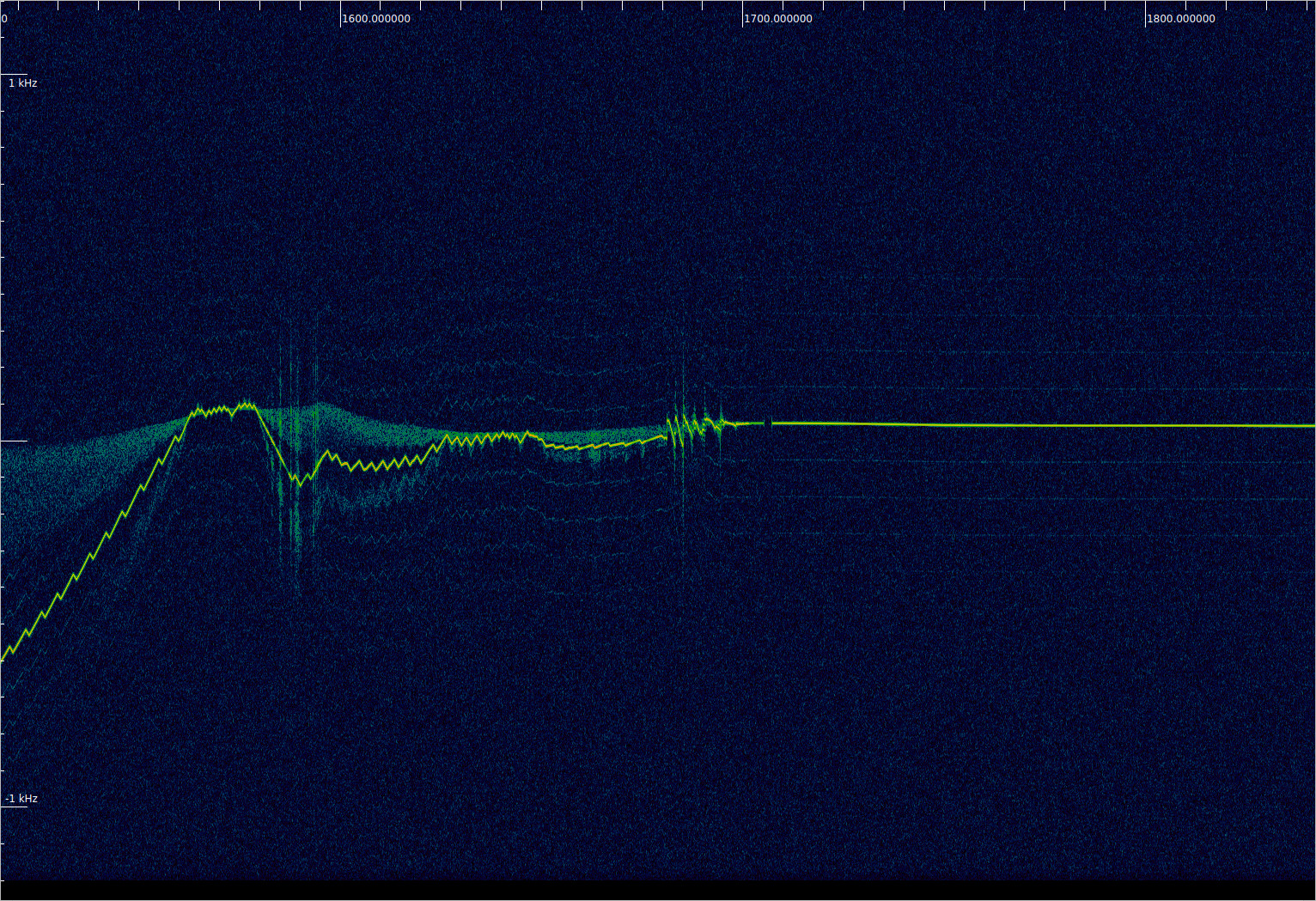
The part after 15:15 UTC is quite interesting, because the residual carrier shows a “triangle wave pattern”. This is best seen in the following Inspectrum waterfall. I think that what happens here is that the thrusters were switched on and off in rapid succession in order to achieve the desired average thrust. SLIM approached the landing zone in a northbound polar orbit, and Shioli crater is on the southern hemisphere, so the Earth was in the northern part of the sky. Accelerations opposing the velocity vector thus pointed away from Earth and caused a negative Doppler drift. Therefore, the downwards parts of the triangle wave correspond to moments when the thrusters are on, and the upwards parts correspond to moments in which the thrusters are off.
The next waterfall shows the moment of touchdown. After this, the transmitter switches off for a short period and then resumes with only the lunar Doppler, indicating that it is stationary on the Moon’s surface. Before this, there is a sawtooth pattern that I don’t know how to interpret. The positive jumps of the signal would correspond to very large accelerations. I have wondered if these frequency jumps are of a non-physical nature. Perhaps the spacecraft receiver’s PLL lost lock. However, the exact same sawtooth pattern also appears in the telecommand signal. This strongly suggests that the receiver PLL was in lock. Since the telecommand signal is transponded at baseband, if the PLL had lost lock, the signal would become “doubled”, as the receiver frequency error would cause the two sidebands of the telecommand signal not to overlap at baseband.
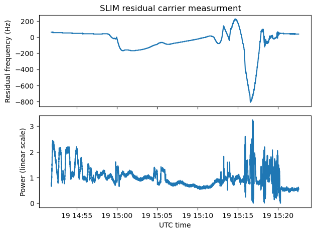
The next plot contains the frequency and power measurements of the residual carrier done using the waterfall. The power of the signal doesn’t change by that much during the whole landing sequence.
Finally, here is a series of plots related to the landing trajectory. There is a lot to unpack here, so I will explain each subplot below the figure. All this data has been computed from the HORIZONS ephemerides.
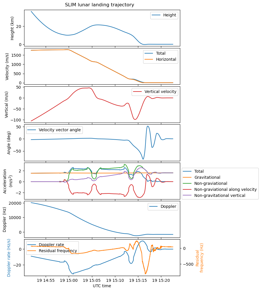
The first subplot shows the height of SLIM above the altitude of the landing zone. Until 15:00 UTC the spacecraft is free falling on an orbit with a periapsis altitude of 10 km. When it passes periapsis, it begins to decelerate and increase its altitude somewhat, before descending again as it continues decelerating. The second plot shows the spacecraft’s total velocity and horizontal velocity. Most of the velocity is in the horizontal component until the final part of the landing, when most of the horizontal velocity has been cancelled out. The third plot shows the vertical velocity.
The fourth plot contains the angle of the velocity vector with respect to the horizon. Until 15:14 the angle is slightly negative, but close to zero, since there is a lot of horizontal velocity. Then the angle becomes increasingly more negative as the spacecraft has cancelled most of the horizontal velocity and is now on a steep powered descent curve. Finally, the angle sweeps up and down due to the vertical velocity alternating between positive and negative some minutes before touchdown.
The fifth plot shows accelerations. The total acceleration (the norm of the acceleration vector) of the spacecraft is shown in blue. The orange curve shows the gravitational acceleration. This depends on the altitude, so it varies slightly as the spacecraft descends. The green curve is the non-gravitational acceleration. This represents the thrust applied by the engines during flight, and also the acceleration exerted by the ground once the spacecraft has touched down. The red curve shows the projection of the non-gravitational acceleration along the velocity vector, and the purple curve is the vertical non-gravitational acceleration.
Looking at the non-gravitational acceleration, we see that there are three distinct phases of thruster firings. We also saw these in the plot of the velocity. The first two phases are mainly intended to cancel a large fraction of the spacecraft’s velocity. Most of the acceleration is along the velocity vector, and opposite to it. The acceleration is about 2 m/s². This is probably the maximum acceleration that the thrusters can achieve. It is enough to counteract the 1.6 m/s² lunar gravity with some margin. In the third phase there starts to be substantial acceleration in the vertical direction, to cancel out the spacecraft’s vertical velocity. The vertical acceleration oscillates around 1.6 m/s², as is needed for a soft landing. It is in this phase when the residual carrier shows a triangle wave pattern that suggests that the thrusters are not fired continuously, but in short bursts.
The sixth plot shows the Doppler that was used in Doppler correction. This resembles somewhat the spacecraft velocity, but it is not the same, since the angle between the velocity vector and the line-of-sight vector changes. The last plot shows a comparison of the Doppler drift and the residual frequency measured on the Doppler corrected residual carrier. Until 15:12 UTC the two curves are quite similar. This suggests that there is a time difference between the Doppler curve used for Doppler correction and what the spacecraft actually did. The difference would be on the order of 5 to 10 seconds, judging by the proportionality of the two curves.
Another thing that we can see is that there are small jumps in the Doppler drift curve. These happen because the HORIZONS ephemerides have discontinuous accelerations. We also saw this in the accelerations plot. Therefore, the Doppler curve that we have used for Doppler correction has some “corners”. We also see these corners in the Doppler corrected signal. Corners in the Doppler correspond to a discontinuous acceleration, which happens when a thruster is suddenly switched on or off. In this case we cannot analyse the Doppler corrected signal qualitatively by looking at the corners that appear, because it is not easy to tell if each of these corners was present in the Doppler correction file, in the original signal, or in both.
It is interesting to compare the data in this post with the telemetry shown in the landing livestream by JAXA, which gives additional context. I hadn’t watched this before, and only watched it after doing the data analysis. I then could realize a few things that I had overlooked in the data. For instance, the non-gravitational acceleration provided by the engine thrust increases somewhat as the mass of the spacecraft decreases due to spent fuel. The livestream also mentions that the thrusters are switched on and off rapidly during the final descent, confirming what we have seen in the Doppler.
The Jupyter notebook and GNU Radio flowgraph used in this post can be found in this repository.
As always – fantastic analysis, Dani !!
Yes, our receivers are all locked to a highly stable 10 MHz reference, RB-Normal, GPSDO locked.