Lunar reflections during SLIM landing

In my previous post, I looked at the Doppler of the SLIM S-band telemetry signal during its landing on the Moon. I showed some waterfall plots of the signal around the residual carrier. In these, a reflection on the lunar surface was visible. The following figure shows a waterfall of the signal around the residual carrier, after performing Doppler correction and using a PLL to lock to the residual carrier. I was intrigued by the patterns made by these reflections, specially by some bands that look like a ‘1’ shape (the most prominent happens at 14:58).

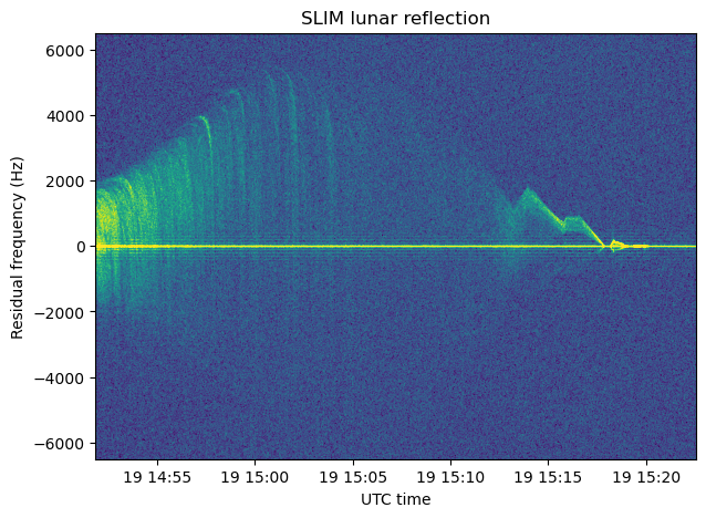
In this post I study the geometry of the lunar reflection and find what causes these bands.

Problem outline

The variable that we have to separate reflections from different points of the Moon’s surface is Doppler. This is only one variable. Since the lunar surface is two-dimensional, the problem of determining where the reflection comes from is undetermined. At any given instant there is a whole curve of points on the lunar surface that all have the same reflection Doppler. However, not all is lost, even if at some instant all the points in these curve have the same reflection Doppler, as time passes the points will have different Doppler versus time curves. So by assuming that there is a certain correlation in reflection strength over time for each point, we might be able to identify individual points on the lunar surface from their Doppler trajectories. Looking back at the figure above, the question becomes: “do the higher intensity patterns in the reflection match the Doppler trajectories of points on the lunar surface?”.

Doppler formulas

Here we are only interested in the frequency difference between a reflected signal and the direct line-of-sight signal. This is what is plotted in the vertical axis of the figure above. We can make some approximations when computing the Doppler of the reflected signal.

An accurate reflection Doppler calculation involves knowledge of the trajectories of the transmitter \(A(t)\) and receiver \(B(t)\) in an inertial frame. Assuming we are able to determine the point \(P(t)\) where the signal that arrives to the receiver at time \(t\) has bounced off (the bounce happens at time \(t – c^{-1}\|B(t) – P(t)\|\)), then the Doppler is\[-\frac{f_c}{c}\frac{d}{dt}\left[\|B(t) – P(t)\| + \|P(t) – A(t – \tau(t))\|\right],\]where \(f_c\) is the carrier frequency and \(\tau(t)\) is the solution to the equation\[\|B(t) – P(t)\| + \|P(t) – A(t – \tau(t))\| = c\tau(t).\]This formulation is complicated to work with, and it also makes the questionable assumption that we are able to meaningfully identify a trajectory \(P(t)\) for the point where the reflection occurs. This makes sense when the reflection happens at a well-defined point, such as the specular reflection point, but not in a more general situation where the reflection is spread over an area.

One approximation that we can make is to ignore the finite propagation speed of light. This amounts to saying that \(A(t – \tau(t))\) is approximately equal to \(A(t)\), which allows us to ignore \(\tau(t)\) completely. In the case of SLIM, \(\tau(t)\) is on the order of one second, and is dominated by the distance between the Moon and the Earth. A more accurate approximation would take a fixed value \(\tau_0\) corresponding to the Moon-Earth distance when the landing happened, and replace \(A(t-\tau(t))\) by \(A(t-\tau_0)\).

Once we ignore the finite propagation speed of light, the reflection Doppler formula involves only points at the same time instant \(t\). Therefore, instead of doing the calculations in an inertial frame, we can do the calculations in a non-inertial frame. In what follows we will ignore the propagation speed of light and assume that \(A(t)\), \(B(t)\) and \(P(t)\) are given in lunar body-fixed coordinates, since this will simplify the calculations.

Since\[\frac{d}{dt}\|v(t)\| = \frac{\langle v'(t), v(t)\rangle}{\|v(t)\|},\]we have that the reflection Doppler is\[-\frac{f_c}{c}\left[\frac{\langle B'(t) – P'(t), B(t) – P(t)\rangle}{\|B(t)-P(t)\|} +\frac{\langle P'(t) – A'(t), P(t) – A(t)\rangle}{\|P(t)-A(t)\|}\right].\]We assume that the vector \(P'(t)\) lies in the plane tangent to the lunar surface at \(P(t)\) (taking into account any surface roughness or inclination), and denote by \(N(t)\) a unit vector normal to this tangent plane. This assumption follows naturally from the condition that \(P(t)\) must lie in the lunar surface for all \(t\). Note that here we are using the fact that \(P(t)\) is given in lunar body-fixed coordinates. Certainly \(P'(t)\) would not lie in the plane tangent to the surface if \(P(t)\) is given in an inertial system centred at the Earth-Moon barycentre. We also assume that the incoming and reflected rays are related by a reflection along this tangent plane:\[\frac{B(t) – P(t)}{\|B(t) – P(t)\|} = \frac{P(t) – A(t)}{\|P(t) – A(t)\|} – 2 N(t) \frac{\langle P(t) – A(t), N(t)\rangle}{\|P(t) – A(t)\|}.\]Since \(\langle P'(t), N(t)\rangle = 0\), this implies\[\frac{\langle P'(t), B(t) – P(t)\rangle}{\|B(t) – P(t)\|} = \frac{\langle P'(t), P(t) – A(t)\rangle}{\|P(t) – A(t)|}.\]Thus, we can simplify the above formula for the reflection Doppler to\[-\frac{f_c}{c}\left[\frac{\langle B'(t), B(t) – P(t)\rangle}{\|B(t)-P(t)\|} -\frac{\langle A'(t), P(t) – A(t)\rangle}{\|P(t)-A(t)\|}\right].\]

Doing a similar reasoning, we can find that the direct line-of-sight Doppler is approximately equal to\[-\frac{f_c}{c}\left[\frac{\langle B'(t), B(t) – A(t)\rangle}{\|B(t)-A(t)\|} -\frac{\langle A'(t), B(t) – A(t)\rangle}{\|B(t)-A(t)\|}\right].\]The vectors \((B(t) – P(t))/\|B(t)-P(t)\|\) and \((B(t) – A(t))/\|B(t)-A(t)\|\) are approximately equal, since the receiver on the Earth \(B(t)\) is much further away from \(P(t)\) and \(A(t)\) than the distance between \(P(t)\) and \(A(t)\), which are points close to the Moon. We are only interested about the difference between the reflection Doppler and the direct Doppler, so we can ignore the first terms in the two formulas above and obtain\[\frac{f_c\langle A'(t), P(t) – A(t)\rangle}{c\|P(t)-A(t)\|}\]for the reflection Doppler and\[\frac{f_c\langle A'(t), B(t) – A(t)\rangle}{c\|B(t)-A(t)\|}\]for the direct Doppler. These formulas have the following interpretation: the reflected Doppler is equal to the projection of the spacecraft velocity vector onto the unit vector that gives the line-of-sight from the spacecraft to the reflection point; the direct Doppler is equal to the projection of the spacecraft velocity vector onto the unit vector that gives the line-of-sight from the spacecraft to the receiver at Earth. For simplicity, we can ignore the location of the receiver on Earth and take as \(B(t)\) the centre of the Earth.

Specular reflection

In a simplified model where the lunar surface is assumed to be flat and the receiver very far away, it is quite easy to compute the specular reflection point. The trajectory of the reflected ray is obtained by reflecting the direct ray along a horizontal plane centred on the transmitter. In particular, the angle that the reflected ray makes with this horizontal plane as it originates from the transmitter is equal to the angle made by the direct ray (but it goes downwards instead of upwards).

In this flat surface model, the difference between the specular reflection Doppler and the direct Doppler has a nice interpretation: it is proportional to twice the vertical velocity of the spacecraft. This is because the vectors from the spacecraft to the reflection point and to the receiver are symmetric with respect to the horizontal plane.

A more accurate model considers the lunar surface as a sphere and does not assume that the distance to the receiver is infinite. I have already treated in this blog the problem of calculating the reflection point on a sphere for a ray travelling between two given points. In the appendix of this post I computed the reflection point as the point that minimizes the length of the reflection path, and solved the minimization problem by brute force. It turns out that this problem is called Alhazen’s problem and it does not have a closed form solution. It can be solved by finding the roots of a quartic polynomial or by numerically solving an equation involving trigonometric functions. This short paper describes these two ways to solve it.

As a comparison of each of the two models, the following plot gives the distance along the lunar surface from the subsatellite point to the specular reflection point calculated with the flat surface and receiver at infinity model and with Alhazen’s problem (spherical surface model). We can see that there is a noticeable difference between the two models at the beginning of the recording, when SLIM is still at 40 km height, but the difference becomes much smaller as SLIM descends.

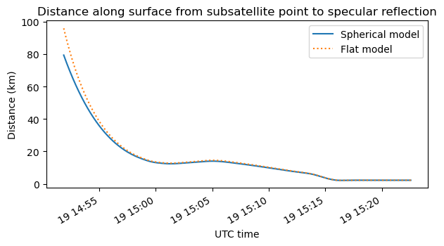
The spherical model predicts a specular point that happens closer to the spacecraft than the flat model. This is because due to the curvature of the surface, the surface normal rotates away from the spacecraft as we go further along the surface. Therefore, compared to a reflection on a flat surface, the ray from the transmitter must be tilted slightly more downwards so that after the reflection on the spherical surface the outgoing ray has the correct angle to reach the receiver.

In the spherical surface model, the difference between the specular reflection Doppler and the direct Doppler is no longer proportional to twice the vertical velocity, but it is reasonably close as long as the spacecraft is not very high. Therefore, this is still a useful intuition to keep in mind.

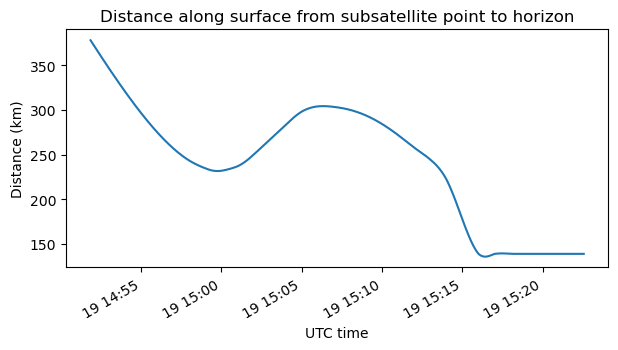
Here is the distance along the surface from the subsatellite point to the horizon, assuming a spherical surface. This gives the radius of the footprint of the satellite. The HORIZONS ephemerides that I’m using for these calculations are not accurate enough after 15:15 UTC. In fact, they give a landing location which is some 5 km above the surface. This is what causes the relatively large distance to the horizon at the end of the plot.

LVLH frame and maximum Doppler

In what follows it is useful to define a LVLH (local velocity local horizon) frame for SLIM. The +Z vector of this frame points up, in the direction of the position vector in Lunar body fixed coordinates. The +Y vector is defined as the cross product of +Z and the velocity vector in Lunar body fixed coordinates. This gives a vector that is normal to the orbital plane. The +X vector is defined as the cross product of +Y and +Z. This gives a right-handed system, and moreover +X points in the direction of the horizontal velocity vector.

The following plot shows the angles that the velocity vector and a vector joining the spacecraft with a point in the horizon make with the horizontal XY plane. We see that for most of the recording the velocity vector points above the horizon. This is in fact what is needed if the spacecraft “wants to miss the ground”. In the final part of the landing the spacecraft initiates a steep descent and the velocity vector now points significantly below the horizon.

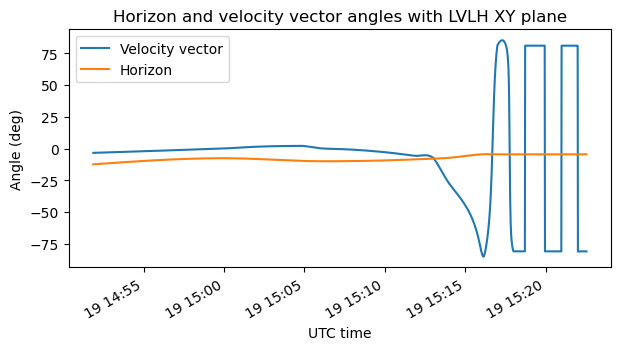
This geometry has implications for the reflection Doppler. As we have seen above, we can approximate the reflection Doppler as the projection of the velocity vector onto the line-of-sight vector to the reflection point. The Doppler is maximal when these two vectors are aligned, but the reflection point needs to be on the surface. When the velocity vector points below the horizon in the steep descent, it points to a spot on the surface that gives the maximum Doppler. When the velocity vector points above the horizon, the spot on the surface that gives maximum Doppler is the point in the horizon ahead of the spacecraft.

The following plot overlays on the waterfall of the signal reflection the Doppler curves corresponding to the specular reflection (computed using the spherical surface model), the maximum Doppler (with the restriction that the reflection point must be on the ground), and the Doppler at the point in the horizon ahead of the spacecraft. The two latter curves coincide for most of the recording, because the velocity vector points above the horizon. Even when they don’t coincide during the steep descent, they are close.

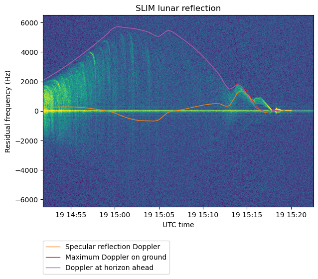
From this plot it is clear that the ephemerides are bad after 15:15 UTC, since the waterfall shows reflections that exceed the maximum Doppler according to the ephemerides. Before 15:15 UTC, the contour of the area in the time-frequency plane where there is a reflected signal matches the maximum Doppler on ground quite well.

Something else is noteworthy. The specular reflection Doppler curve doesn’t have any reasonably obvious counterpart in what we see in the waterfall of the signal (except perhaps during the steep descent some minutes before 15:15 UTC). This means that most of the reflected signal power that we see doesn’t correspond to the specular reflection. This contrasts with the lunar reflections that we saw from the Lonjiang-2 mission at UHF, which followed the specular reflection Doppler curve quite well. Some reasons why the specular reflection is not prominent in this case will be given below.

A particular reflection

The thing that intrigued me most in the waterfall of the reflected signal is the curved shapes that look like a ‘1’. The clearest of these happens at 14:58 UTC. Maybe these correspond to reflections on some specific parts of the lunar surface. But which parts? And why do these parts produce a stronger reflection?

What I have done to answer these questions is to try to match the shape in the waterfall with the Doppler curve of a particular point in the Moon surface. The way in which I chose this point is by specifying the moment in which the point is in the horizon (this is the moment in which the point first becomes visible from the spacecraft, and so a reflection can start to happen), and the heading to this point in this moment (using the LVLH frame introduced above). By varying these two parameters I try to match the Doppler curve with the shape on the waterfall. Roughly speaking, changing the time at which the point appears on the horizon moves the curve left or right, and changing the heading to the point when it is in the horizon affects the amplitude and steepness of the curve. I also consider points that appear in the horizon at a slightly earlier and later times, and at a slightly smaller and larger heading, in order to obtain some error bars for the location of the point.

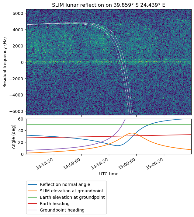
The following figure shows a plot of the strongest of these shapes (the one happening at 14:58 UTC), and the Doppler curve for a point in the surface that matches this shape, as well as the two error bars. The latitude and longitude of the reflection point is given in the figure title.

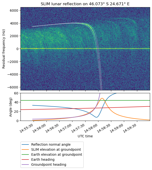
There is a lot to unpack in the plot below the waterfall, so let’s go curve by curve. The blue curve shows the value that the angle between the normal of the reflection plane and the vertical must have so that the reflection can happen. This is not a specular reflection, so the angle is not zero, the surface causing the reflection must be tilted with respect to a perfect spherical surface in order to allow for the reflected ray to reach the Earth. We see that the angle ranges between 10 and 20 degrees when the reflection is strongest.

The orange curve gives the elevation of SLIM as seen from the reflection point. This starts at zero when the point first appears on the horizon of SLIM, increases to a maximum as SLIM passes abeam of this point, and then decreases again as SLIM leaves the point behind and it disappears below the horizon. The green curve is the elevation of Earth as seen at the reflection point. This will become relevant below.

Finally, the red and purple curves give the heading from SLIM to Earth and to the reflection point. The heading is defined with respect to the LVLH frame defined above. Due to how the frame is defined, heading increases counterclockwise, instead of clockwise as is more usual. As a general rule, in order for a strong reflection to happen, the transmitter, reflector and receiver need to be more or less aligned. These means that the two headings must be close. A reflection plane that is very tilted can provide a reflection path in which the heading changes significantly. Also, scatter by a rough surface (which can be modelled as the surface normal varying quickly at a small scale) can change the heading of a reflection. But usually the reflection cannot change the heading much. We see that the reflection is only strong when the difference between the two headings is less than 10 degrees or so. This matches our intuition.

An important remark is that points that are symmetric with respect to SLIM’s groundtrack give the same reflection Doppler curve. This happens because the angles between SLIM’s velocity vector and the line-of-sight vector from SLIM to each of these two symmetric points always coincide. Here the point I have selected is west of SLIM’s groundtrack. The Earth is also west of SLIM, since SLIM is travelling towards the north in the eastern hemisphere of the Moon. Therefore, at some instant this point on ground, and Earth become aligned. There is a symmetric point east of SLIM’s groundtrack that has the same Doppler curve. This point has opposite heading to that of the point we’re considering. The heading difference for this point is therefore always large, and so a strong reflection at this point cannot happen.

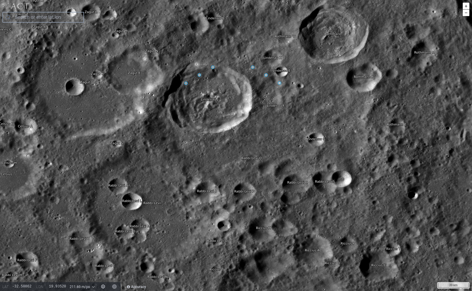
The figure below shows the reflection points plotted in LROC QuickMap. Six points are shown: the reflection point west of SLIM and the two points used as error bars, and the symmetric point east of SLIM with its two error bar points. When the reflection is most strong, SLIM was south of these points, seeing the points at a heading between 10 and 20 degrees, and travelling north. The Earth would be to the northwest, at a heading slightly above 20 degrees.

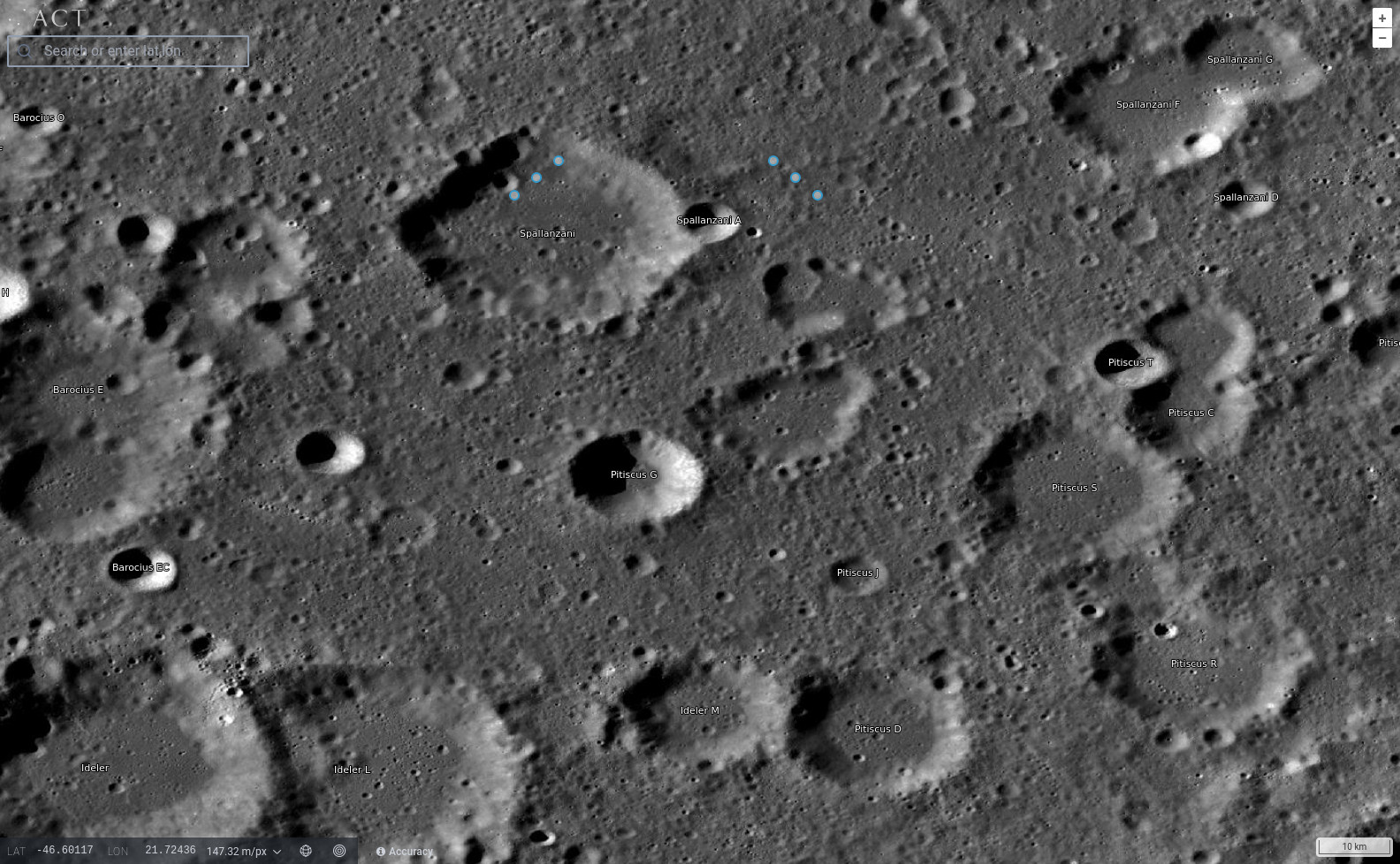
It is remarkable that the points west of SLIM fall quite close to the nortwestern wall of Spallanzani crater. If we imagine the geometry, the Earth is at an elevation of around 45 degrees at this point of the lunar surface. When the reflection is strongest, SLIM is lower on the sky of the reflection point, at an elevation of around 20 degrees. The northwestern wall of the crater, with a slope of around 20 degrees is exactly what is needed to reflect the SLIM signal upwards towards Earth, instead of to a lower elevation, as a flat surface would do. The SLDEM2015 slope data in QuickMap shows that the slope of this crater wall ranges between 15 and 30 degrees, so it provides many surfaces that have the required geometry for the reflection to happen.

Other reflections

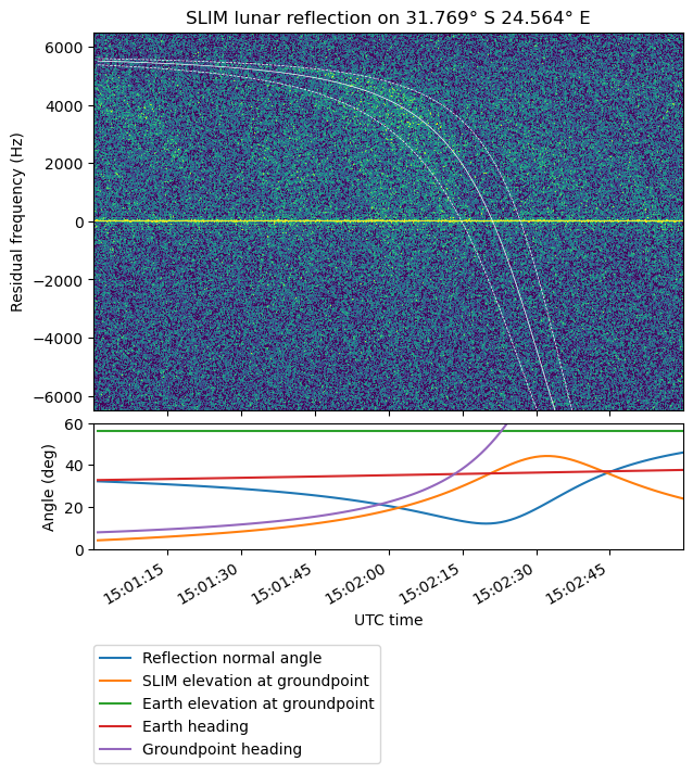
The surface point whose reflection Doppler curve was a good match for the reflection shown above is very close to the northwestern wall of a crater. I have explained why this situation should give a good reflection geometry, but to try to find if this was just a coincidence, I have studied some of the other reflections that are distinctly visible in the waterfall. Their plots are shown here.

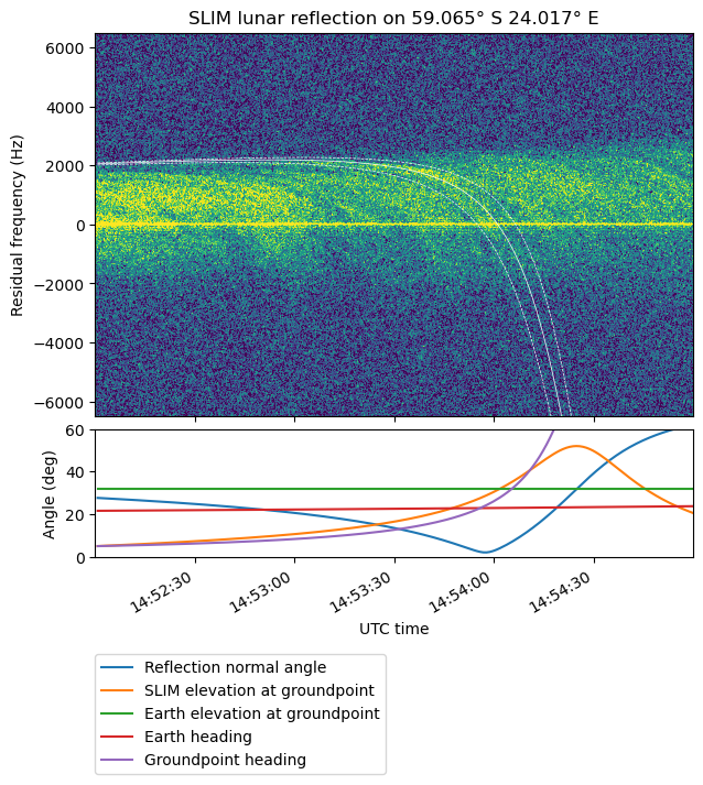
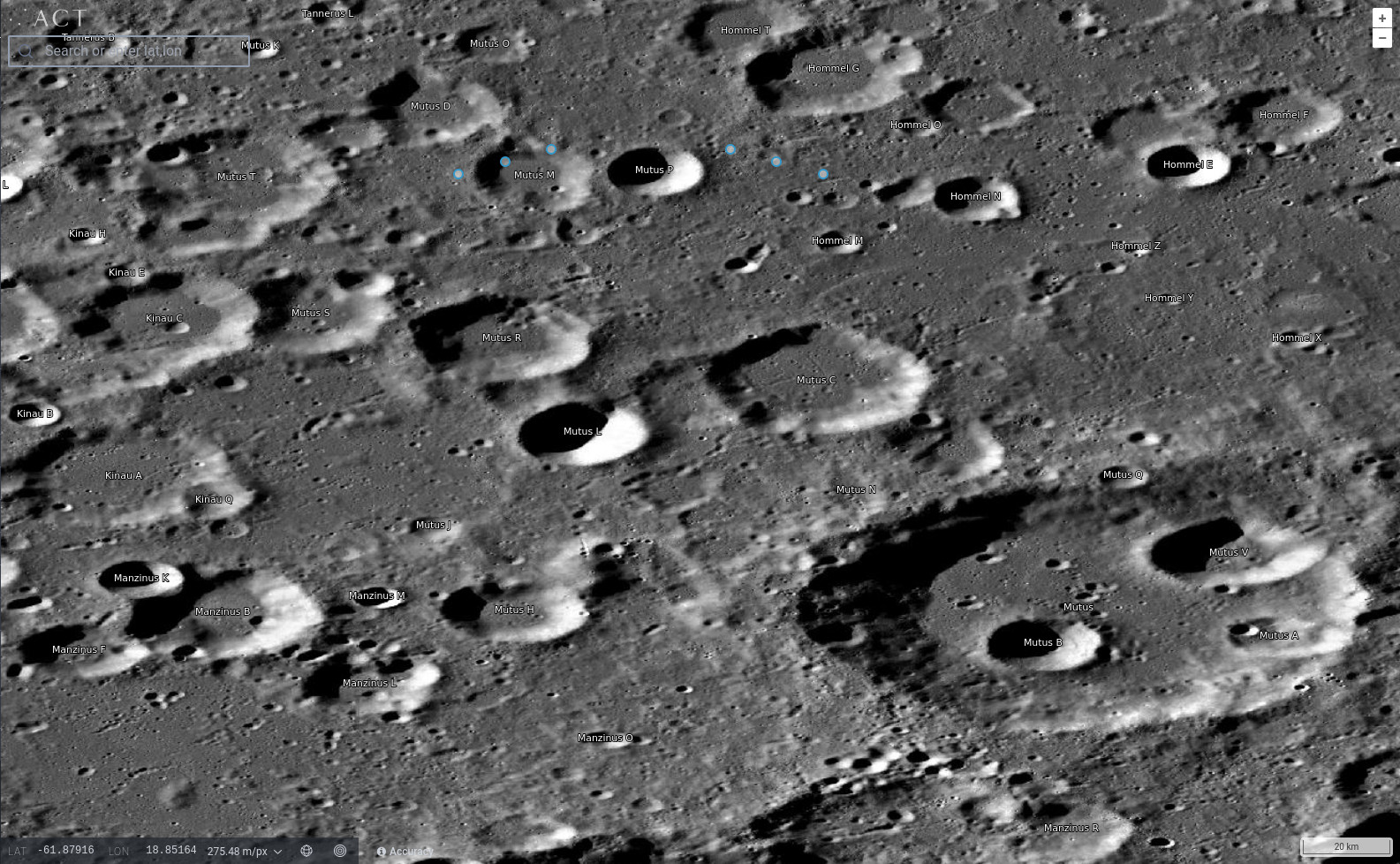
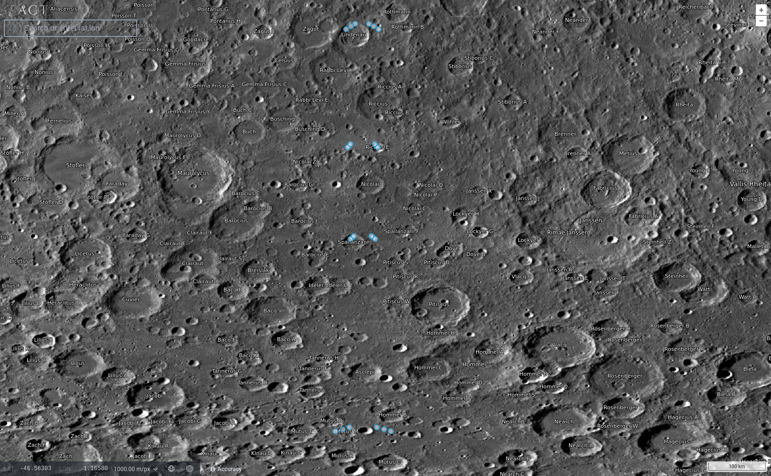
To automate the analysis with QuickMap, I’m exporting the reflection points in a GeoJSON, which can then be loaded in QuickMap. The first of these reflection points is at the northwestern wall of the Mutus M crater.

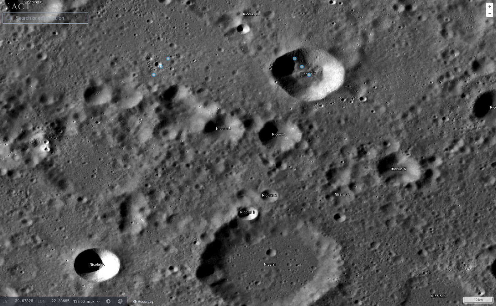
The next reflection is more difficult to explain. The reflection point lies somewhat north of the wall of a crater next to Nicolai E. It might be that this wall is what causes the reflections. There are several smaller craters around the reflection point, and these also provide a surface normal which is as required by the reflection geometry. Interestingly, the symmetric reflection point east of SLIM lies inside a crater, although I don’t think that this crater can turn the heading of the reflection path by around 40 degrees, which is what would be needed to get a reflection there.

Finally, the reflection point for the last reflection matches quite well the northwestern wall of the Lindenau crater.

The following map shows all the reflection points that I have identified. This gives good evidence for the fact that a distinct reflection appears in the waterfall whenever SLIM passes southeast of a crater, as the northwestern crater wall gives a surface that can reflect the signal upwards to Earth.

Polarization

A natural question is why the specular reflection is missing in the waterfall plot. The relatively flat lunar surface between the craters provides ample opportunities for a specular reflection to happen. Something to keep in mind is that the polarization used for this recording is the one corresponding to the direct signal (nominally RHCP). How a reflection interacts with circular polarization depends on the incidence angle. A normal reflection returns circular polarization of the opposite sense. This is well know when dealing with antenna reflectors. In contrast, a grazing reflection returns circular polarization of the same sense. In general a mixture of RHCP and LHCP will be returned depending on the incidence angle. When the incidence matches Brewster’s angle, the return will be horizontally polarized. This can be understood as 50% RHCP and 50% LHCP.

The report Radar Reflectivity of the Earth’s surface by Katz gives more details about this. The exact behaviour depends on the surface composition and frequency, but qualitatively it is always as described above. The following figure, taken from this report, gives the reflection coefficients for a smooth sea surface at a frequency of 6 GHz. In the case of SLIM we instead have the lunar surface at 2.1 GHz. I don’t know if the S-band reflectivity of the Moon has been studied in this detail.

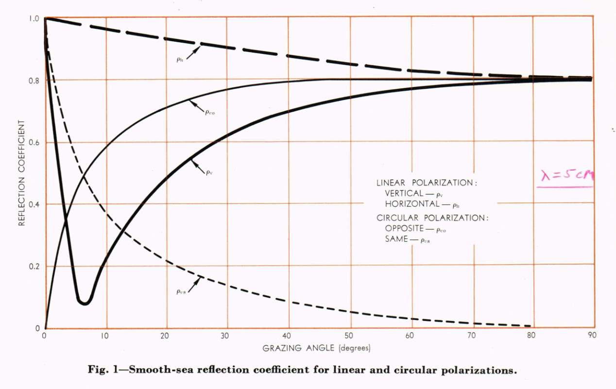
The reflection coefficient for circular polarization is given by the thin lines. Same-sense polarization is the dashed line, and opposite-sense polarization is the continuous line. We see that there is only a large same-sense reflection for small grazing angles. In this case the Brewster angle is around 7 degrees. There is still some small amount of vertical polarization returned at this angle, probably because the surface does not behave as an ideal model.

In the case of SLIM, the grazing angle for a specular reflection is equal to the elevation of the Earth at the reflection point. This elevation increases as SLIM travels north through the southern lunar hemisphere, but in general it ranges between 35 and 60 degrees. These angles are probably well above the Brewster angle, so only a small fraction of same-sense polarization power is returned. I think this explains why there is no distinct sign of a specular reflection in the waterfall plot. It would have been very interesting to record this event in dual polarization and compare the two polarizations.

Even if we consider non-specular reflections, the grazing angle is bounded below by the geometry. Since SLIM must be at a non-negative elevation at the reflection point, the minimum grazing angle is \(\varepsilon_E/2\), where \(\varepsilon_E\) is the elevation of Earth at the reflection point. More in general, the grazing angle is \(\varepsilon_E/2 + \varepsilon_S/2\), where \(\varepsilon_S\) is the elevation of SLIM at the reflection point. This shows why the same-sense polarization waterfall favours reflections far from SLIM, for which \(\varepsilon_S\) is small. Such reflections need a surface slope of \(\varepsilon_E/2 – \varepsilon_S/2\) in order to reflect the signal upwards towards Earth. Since the heading to the reflection point and the heading to Earth must also be close, this means that the same-sense polarization waterfall favours reflections on a direction which is close to the velocity vector. These have a Doppler that is larger than the specular reflection or the direct signal.

We can also see that the reflection in general gets weaker as time advances, until the moment of the steep descent. This makes sense taking polarization into account. As SLIM travels further north, the Earth is higher up on the sky, so it is more difficult to get reflections with small grazing angle that have a significant amount of sense-sense return. There is another effect that is at play here, since SLIM is also descending. This means that the area that can reflect signals gets smaller, as the footprint shrinks. On the other hand, there is less free-space path loss in the radar equation. It turns out that the free-space path loss reduction wins out, so in general a lower height should give more reflected power.

This is not the full story of why of all the possible non-specular reflection paths only some of them are strong in the waterfall. The transmitter antenna pattern would also play a role here, but I don’t have any information about this. At least we know that until the steep descent the attitude of the spacecraft was more or less the same, since it was pointing the engine for a retrograde burn. When the steep descent happens, the attitude changes significantly. Perhaps this explains why a strong reflection appears again, even though the Earth is now very high in the sky and reflections with small grazing angle are not possible.

Conclusions

In this post I have shown how some distinct patterns in the waterfall of the signal reflected off the Moon’s surface during SLIM’s landing can be matched to the Doppler curves of reflections happening on the northwestern walls of craters. As SLIM passes southeast of these craters while travelling north on the southern lunar hemisphere, these walls give the required reflection geometry. Moreover, compared to the specular reflection, these reflections on crater walls have a significantly smaller grazing angle, which causes a higher same-sense polarization return.

The fact that the data was only recorded in same-sense polarization constrains the area where stronger reflections can happen, favouring this kind of crater wall reflections. How the transmitter antenna pattern illuminates the lunar surface also influences which reflections can be strongest, but there is not enough data about the transmitter antenna to use this in the interpretation of the observation.

Code and data

The Jupyter notebook and GNU Radio flowgraph used in this post can be found in this repository.