If you have been following my latest posts, you will know that a series of observations with the DSLWP-B Inory eye camera have been scheduled over the last few days to try to take and download images of the Moon and Earth (see my last post). In a future post I will do a chronicle of these observations.
On October 6 an image of the Moon was taken to calibrate the exposure of the camera. This image was downlinked on the UTC morning of October 7. The download was commanded by Reinhard Kuehn DK5LA and received by the Dwingeloo radiotelescope.
Cees Bassa observed that in the waterfalls of the recordings made in Dwingeloo a weak Doppler-shifted signal of the DSLWP-B GMSK signal could be seen. This signal was a reflection off the Moon.
As far as I know, this is the first reported case of satellite-Moon-Earth (or SME) propagation, at least in Amateur radio. Here I do a Doppler analysis confirming that the signal is indeed reflected on the Moon surface and do some general remarks about the possibility of receiving the SME signal from DSLWP-B. Further analysis will be done in future posts.
Below you can see the tweet where Cees Bassa reported the Moonbounce signal. As you can see, it is an awesome result indeed, only achievable with large dishes such as Dwingeloo’s. He even “challenged” me to decode the Moonbounce signal. I think that the signal is too weak for the Turbo decoder to wipe all bit errors, but perhaps I will try something in a future post.
The figure below shows the direct path and Moonbounce Doppler for the 436.4MHz downlink signal of DSLWP-B, as seen in the groundstation at Dwingeloo, for the timespan of the recordings done on the morning of October 7.
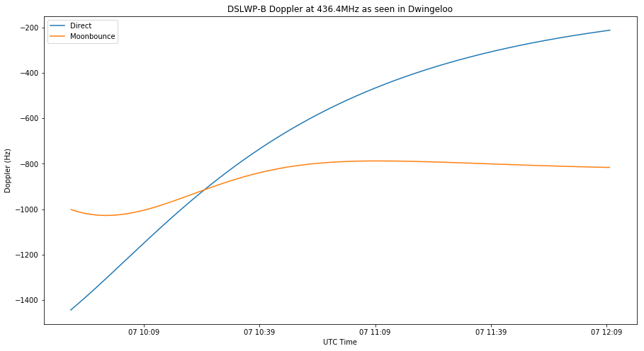
The direct path Doppler is computed as usual by using GMAT to output the position and velocity of DSLWP-B in a topocentric frame of reference centred at Dwingeloo and calculating the Doppler as the projection of the velocity vector onto the line-of-sight vector (see this post). Computing the Moonbounce Doppler is not as easy as it might first seem. The details are included in an appendix below.
The figures below show the waterfalls of the recordings of the 436.5MHz signal overlaid with the direct and Moonbounce Doppler curves. The waterfalls have been shifted -750Hz to correct for the frequency offset in the local oscillators of DSLWP-B and the receiver in Dwingeloo, so that the direct Doppler curve matches the received signal.
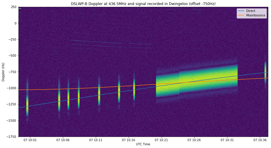
In the figure above we see that there is a visible Moonbounce signal at the beginning of the recording. Then the difference between the direct and Moonbounce Dopplers is too small to tell the two signals apart.
We can also observe a frequency jump in the DSLWP-B TCXO in the long transmission, which contains the SSDV packets. These TCXO jumps have already been documented and they explain some of the losses of SSDV packets.
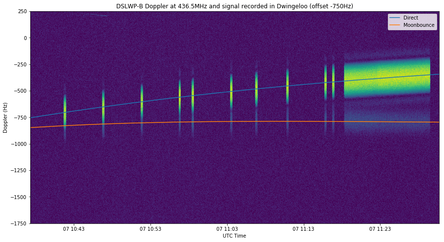
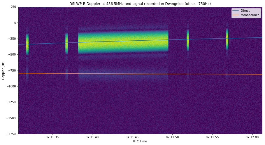
In the two figures above the difference between the direct and Moonbounce Dopplers is large and the Moonbounce signal can be seen almost all the time in the waterfall.
The three figures below contain the recordings of the 435.4MHz signal made at Dwingeloo. The Moonbounce signal is weaker, so Cees hadn’t noticed it, but with the help of the Doppler curve it can be seen sometimes.
The 435.5MHz signal alternates between GMSK and JT4G beacon transmissions. The lowest tone of the JT4G signal is 1kHz above the GMSK signal, and the tone separation is 312.5Hz. I have included lines marking the expected frequencies of each of the four JT4G tones, according to direct or Moonbounce Doppler.
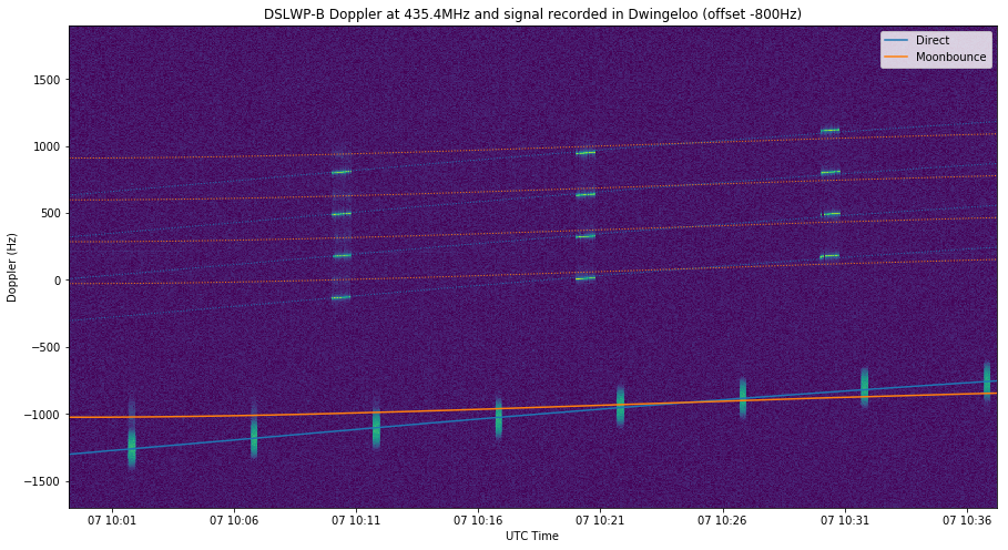
At the beginning of the recording shown in the figure above, we have a visible reflection of the GMSK signal. Also, a reflection of the first JT4G signal is barely visible. It seems to show some Doppler spread.
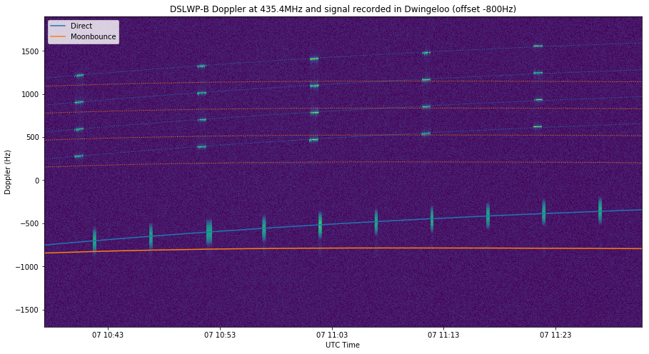
In the figure above, faint reflections of the GMSK signal can be seen near the centre of the recording.
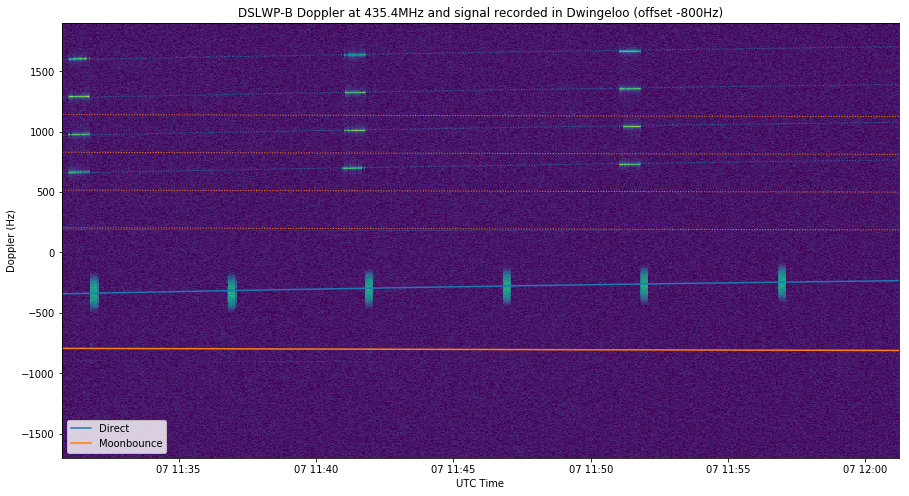
No reflections can be seen in the last 435.4MHz recording, shown in the figure above.
For a rough comparison of the signal strengths, I have extracted the beginning of the SSDV transmission in the second recording of the 436.4MHz signal and used my GMSK detector with the direct and Moonbounce signal (I have used a low pass filter in Audacity to remove the direct signal to force the GMSK detector to choose the Moonbounce signal). The results are shown below.
Direct signal:
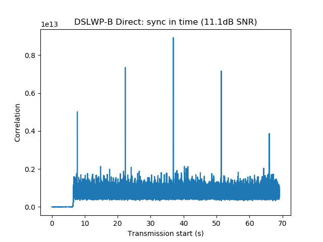
Start time: 36.86s Frequency: 346.8Hz CN0: 45.1dB, EbN0: 21.1dB, SNR (in 2500Hz): 11.1dB
Moonbounce signal:
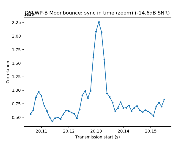
Start time: 20.13s Frequency: 8.1Hz CN0: 19.3dB, EbN0: -4.6dB, SNR (in 2500Hz): -14.6dB
Even thought the GMSK detector doesn’t detected the same packets (note the different start times), we see that there is a difference of roughly 25dB between the direct and reflected signals.
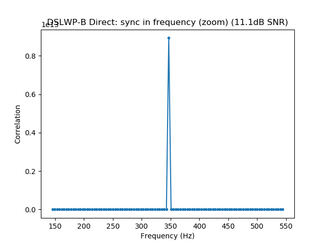
The figures below show the correlation in sync and frequency generated by the GMSK detector with the direct signal. The ASMs are clearly visible and the sync in frequency is very sharp. Note that the resolution in time is on the order of 1ms (or 300km) and the resolution in frequency is on the order of 5Hz.
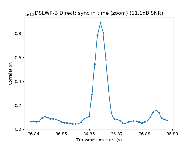
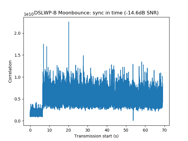
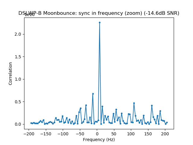
The figures below show the correlations in time and frequency for the Moonbounce signal. Only the first and second ASM are clearly visible. The sync in frequency is still sharp. With the results of these correlations, there is no indication of Doppler spread, so it seems that the reflection happens in a specular manner over a relatively small area of the lunar surface.
In the future I would like to study the cross-correlation of the direct signal (which has a large SNR) against the Moonbounce signal. This might shed more light into whether there is any Doppler or time spread of the Moonbounce signal, indicating a weaker diffuse reflection over a larger area of the lunar surface. Another interesting by-product of this study would be the measurement of the excess path length of the reflected signal, allowing its comparison with the geometry described in the appendix below.
As a final remark, let us compare the path loss of the direct and Moonbounce paths. At a frequency of 436MHz and a distance of 380000km, the free space path loss is -196.8dB. This can be taken as a good estimate for the path loss of the direct path.
The bistatic radar equation shows that the path loss for the reflected path is\[L = \frac{\lambda^2 \sigma}{(4\pi)^3d_1^2d_2^2},\]where \(\lambda\) is the wavelength, \(\sigma\) is the radar cross-section of the reflector, and \(d_1\) and \(d_2\) are the distances between the transmitter and the reflector and between the receiver and the reflector respectively.
As a typical example of the Moonbounce geometry for DSLWP-B we can take \(d_1 = 10000\text{km}\) and \(d_2 = 380000\text{km}\). The radar cross-section of the Moon at a wavelength of 70cm,as seen from the Earth, is estimated as 0.07 times its physical area. The physical area of the side of the Moon visible from Earth is \(9.49\cdot10^{12} \text{m}^2\). Disregarding the fact that we are assuming that the reflection occurs only over a much smaller area of the surface, and using this value as physical area, we have a radar cross-section of \(\sigma = 6.64\cdot10^{11} \text{m}^2\).
Therefore, the estimated path loss of the Moonbounce path is -218.6dB. This means that the Moonbounce path is 21.8dB weaker than the direct path. Taking into account the fact that we have done a very rough estimate for the radar cross section of the reflection area, this fits nicely with the difference of 25dB that we have measured.
Thus, in theory, the Moonbounce signal of DSLWP-B should be receivable by large stations such as Dwingeloo that are able to receive the direct signal with an excess SNR of 25dB, given the right geometric conditions for the reflection. As a comparison, note that the EME path loss at 436MHz is -250.2dB. This is 31.6dB less than the path loss for SME in lunar orbit, and it explains why it is much easier to receive lunar orbit SME than EME. A transmitter on Earth with the same EIRP as DSLWP-B (around 1W) would be virtually impossible to receive in Dwingeloo via EME.
The calculations in this post have been done in this Jupyter notebook and using this GMAT script.
Appendix: Computation of the Moonbounce Doppler
As a rough approximation to compute the Doppler of the Moonbounce path, one is tempted to take the path from DSLWP-B to the centre of the Moon and then from the centre of the Moon to Dwingeloo to compute the Doppler. Then the Moonbounce Doppler would be the sum of the DSLWP-B Doppler, as seen from the centre of the Moon, plus the Doppler of the centre of the Moon, as seen from Dwingeloo. Both of these quantities are easy to compute as we have done with the direct path Doppler.
However, one now may ask what happens when the centre of the Moon is replaced by a particular point on the lunar surface. It turns out that the Doppler curve depends a lot on which point is chosen. This is not so surprising. Since DSLWP-B is relatively close to the Moon, as it orbits, some points of the lunar surface see DSLWP-B approaching and others see it receding. Thus, different points of the lunar surface see DSLWP-B with rather different Dopplers.
Therefore, to have any chance of computing the Doppler of the Moonbounce signal that we have observed in Dwingeloo’s recordings, we first need to determine the point of the lunar surface where the reflection happens. To this end, we assume that the reflection is specular. Approximating the shape of the Moon by a sphere, we are lead to the following interesting mathematical problem.
Let \(A\) and \(B\) be points in \(\mathbb{R}^3\) and \(S\) a sphere such that the line segment joining \(A\) and \(B\) lies outside of \(S\). Prove that there is a unique point \(P \in S\) such that a ray from \(A\) to \(P\) reflects off \(S\) and passes through \(B\). Compute the point \(P\).
This problem can be reduced to the plane by noting that the point \(P\) and the ray should lie in the plane which contains \(A\), \(B\) and the centre of \(S\). Then we can assume that \(A\) and \(B\) are in \(\mathbb{R}^2\) and \(S\) is a circle. Still, it is not so easy to compute the coordinates of a point \(P\) satisfying the needed conditions (one can write a system of two non-linear equations).
An alternative approach is to consider an ellipse \(E\) whose foci are \(A\) and \(B\). If \(P \in E\) and a ray from \(A\) to \(P\) reflects off the ellipse \(E\), then it is known that it passes through \(B\) because of the properties of ellipses. If we can arrange so that the ellipse \(E\) is tangent to \(S\) and define \(P\) as the point of tangency, then the point \(P\) would satisfy the needed conditions, because the reflection off \(S\) at \(P\) is the same as the reflection off \(E\) at \(P\), since these two curves are tangent at \(P\).
Recall that the ellipse \(E\) can defined as the set of points \(Q\) such that \(|Q-A| + |Q-B| = k\), where \(k\) is a positive constant. If we consider the family of ellipses obtained by varying the parameter \(k\), we see that if \(k\) is small enough, then the \(E\) will not intersect \(S\). If we make \(k\) larger, eventually \(E\) will intersect \(S\). The smallest such \(k\) so that \(E\) intersects \(S\) gives an ellipse tangent to \(S\).
Looking at this analysis in another way, we see that the point of tangency \(P\) is the point \(P \in S\) that minimizes the sum of distances \(|P-A|+|P-B|\). From this characterization, the uniqueness of \(P\) follows and it also tells us a way to compute the point of tangency \(P\).
Turning back to our problem about computing the Moonbounce Doppler, we note an additional difficulty. As time passes, the relative positions of the spacecraft, the Moon and the groundstation at Dwingeloo change, so the reflection point \(P\) moves along the Moon surface. Therefore, the velocity of the point \(P\) should also be taken into account when computing the Doppler.
Actually it is easier to organize the computations by writing the Doppler in terms of the time derivative of the propagation path distance. The Doppler equals\[-\frac{f}{c}\frac{d}{dt}(|P-A|+|P-B|).\]
I have done the calculations in probably the least clever way, since I wanted to have this running quickly. We work with the list of positions of DSLWP-B and the Moon in a topocentric frame of reference centred in Dwingeloo. For each timestamp, the point \(P\) is found by searching the point that minimizes the sum of distances \(|P-A|+|P-B|\) where \(P\) runs along a fine grid of points on the Moon surface (actually the point \(P\) is not computed explicitly, since we only need to obtain the minimum sum of distances).
The grid of points on the lunar surface for the minimization is built by taking a grid of points equally spaced in latitude and longitude, so the grid is far from being uniformly distributed over the lunar surface. A grid size of 1000×1000 points seems to work well enough.
The time derivative of the propagation path distance is approximated as the difference quotient between two consecutive timestamps. To give a smooth result, the time step in GMAT is limited to a maximum of 10 seconds.
This algorithm seems to work well, as it generates a smooth Doppler curve that matches the observations. It is interesting to note that the Doppler in this case tells us something about the geometry of the reflection. We see that most of the reflection follows the path that a specular reflection would take.
It is also possible that part of the energy is reflected in a non-specular manner, bouncing off other points on the lunar surface and causing a Doppler spread. It is difficult to judge whether this effect happens just by looking at the waterfalls of the recordings.
8 comments