In one of my latest posts I commented on the Moonbounce signal of the Chinese lunar satellite DSLWP-B, as received in Dwingeloo. In the observation made in 2018-10-07 Cees Bassa discovered a signal in the waterfall of the Dwingeloo recordings that seemed to be a reflection off the Moon of DSLWP-B’s 70cm signal. My analysis showed that the Doppler of this signal was compatible with a specular reflection on the lunar surface.
In this post I study the cross-correlation of the Moonbounce signal against the direct signal. This gives some information about how the radio signals behave when reflecting off the Moon. Essentially, we compute the Doppler spread and time delay of the Moonbounce channel.
In the previous post we’ve seen that the reflected signal was weak, barely visible over the noise floor. Still, we can compute the cross-correlation between the reflected and direct signals. The calculations have been done in this Jupyter notebook.
The cross-correlation algorithm I have used can be summarised by the following formula:\[(x \star y)_k(\tau, \omega) = \sum_{j = 0}^{M-1} |\mathcal{F}_N^{-1}[z_{k+js,\omega}](\tau)|^2,\]where\[z_{k,\omega} = \mathcal{F}_N(x(n+k)w(n) e^{i\omega n} )\overline{\mathcal{F}_N(y(n+k) w(n))},\] and \(x,y\) are the direct and reflected signals respectively, \(\tau\) is the time delay, \(\omega\) is the frequency, \(k\) is the starting sample for the correlation calculation, \(\mathcal{F}_N\) denotes an \(N\)-point DFT, and \(w\) is a window function.
The parameter \(s\) determines the DFT overlap. An usual choice which we will use here is \(s = N/2\), which means that half of the points of one DFT overlap with the next one.
The parameters \(N\) and \(M\) give the so-called coherent integration length and non-coherent integration length. We say that the coherent integration length is \(N\) samples and the non-coherent integration length is \(M(s-1) + N\) samples (or that we do \(M\) non-coherent integrations). The choice of the coherent and non-coherent integration lengths is important because it determines the SNR of the correlation, the frequency resolution and the computational cost. It is also related to the frequency stability of the signal: unstable signals do not get an SNR gain when doing longer coherent integrations.
The recordings made at Dwingeloo use a sampling rate of 40ksps. After several trials I have decided to set a coherent length of \(N = 2^{16}\) samples, or 1.64 seconds. I have chosen \(M = 20\), which gives a non-coherent length of 17.2 seconds.
The window \(w\) I have chosen is the flattop window, which has minimal scalloping loss.
I have decided to make a video with the values of the correlation \((x \star y)_k(\tau,\omega)\). The variable \(k\) is represented by the time of the video, and each video frame represents the values of \((x \star y)_k\) using a colour scale. The horizontal axis represents the delay \(\tau\) and the vertical axis represents the frequency \(\omega\). The index \(k\) is incremented by \(N/2\) samples for each frame, so the frames are \(k = 0, N/2, N, 3N/2, \ldots\)
To give a smoother response in the video, I have modified slightly the definition of \(x \star y\) to include a window \(v\) as\[(x \tilde{\star} y)_k(\tau, \omega) = \sum_{j=0}^{M-1} |\mathcal{F}_N^{-1}[z_{k+js,\omega}](\tau)|^2 v(j).\]The window I have chosen as \(v\) is the Hann window.
The video is played back at 12 frames per second to get a rate which is approximately 10 times faster than real time (actually we get 9.83 seconds of real time per second of video). Each of the videos takes approximately 40 minutes to generate on my computer.
If you recall from the previous post, there were two SSDV transmissions done at 436.4MHz which showed a Moonbounce signal. Each of the transmissions lasts for approximately 10 minutes. One of the transmissions started at 11:17 UTC and the other one at 11:38 UTC. I have done a separate analysis and a separate video for each transmissions. The videos can be seen below.
The span of the horizontal axis of the video is from -600 to 600 samples. Taking into account the speed of light, this is \(\pm 4497\)km. The centre corresponds to no delay (the reflected signal arriving at the same time as the direct signal), so we expect the correlation to appear slightly to the right, corresponding to the extra length that the reflected signal travels (more on this later).
The span of the vertical axis is from -50Hz (bottom) to 50Hz (top). We can see that the signal is spread in frequency more or less randomly over approximately 50Hz.
We can see in the videos that the frequency of the reflections has a chaotic behaviour as the satellite orbits and the reflection path changes slightly. Strong reflections sometimes appear up to \(\pm 25\)Hz from the centre frequency, which represents the Doppler predicted by the specular reflection on a sphere model (see the previous post). Other than the fact that the signal in the second video is slightly weaker than in the first one, we do not see any major difference between both.
Summing up all the correlations (which corresponds to taking \(M\) very large), we obtain the average pattern for the delay and Doppler spread. This is shown in the figures below.
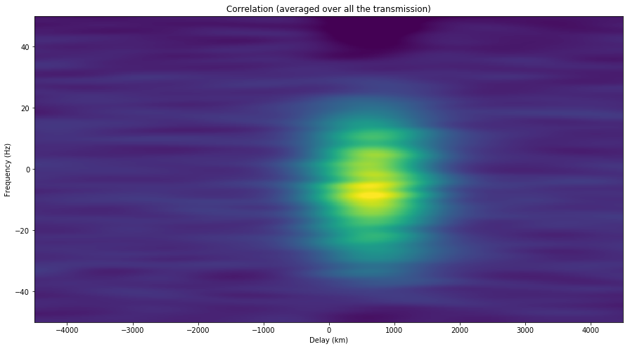
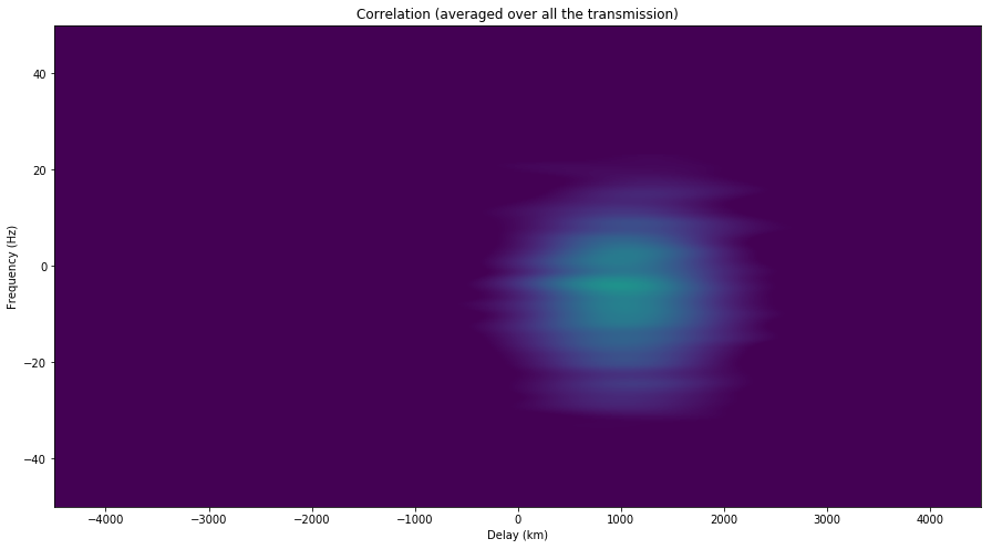
In the figures below, we now sum along the frequency axis to obtain the correlations depending on delay only. We see that the delay of the second transmission is slightly larger than for the first one.

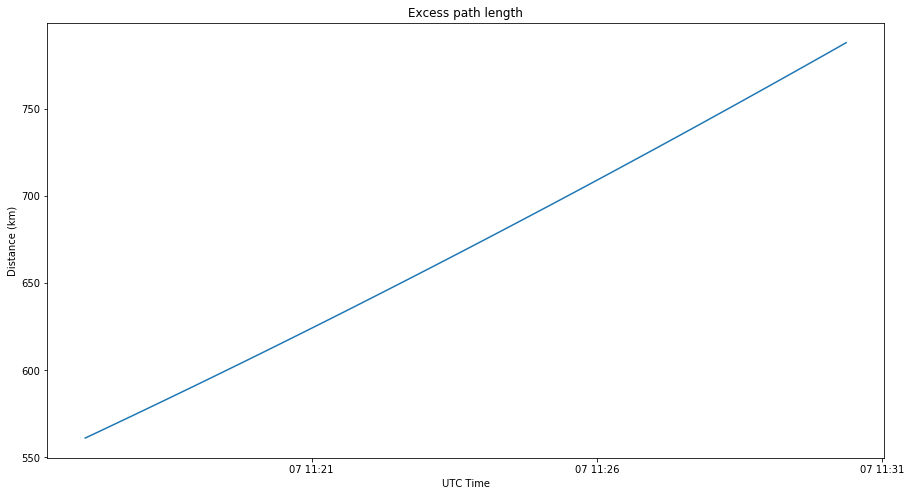
As we have mentioned above, the delay of the reflected signal corresponds to the excess path length travelled, in comparison with the direct signal. Assuming the specular reflection model, the excess path length is shown in the figure below (calculation in this Jupyter notebook).

The figure below shows the excess path length during the first transmission. We see that its value is centred approximately on 675km and that it only changes by approximately 200km during the whole 10 minute transmission. This change is small in comparison with the correlation peak (a symbol at 250baud is 1200km), so the correlation peak is smeared only very little by summing up over the whole transmission without correcting for the change in delay, as we have done above.
The figure below shows the excess path length during the second transmission. The average is around 1075km and the change is 250km.
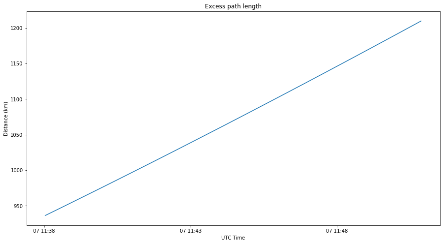
The peaks of the correlations occur at a delay of 660 and 1042km, which match quite well the excess path length model shown above.
If instead of summing up over the frequency axis we sum up over the delay axis, we obtain the energy spectral density of the Doppler spread of the reflected signal. This is shown in the image below. I find it quite interesting that the shape of the spread fits quite well a triangle. It is also interesting that the spread is not centred on 0Hz (which represents the frequency predicted by the specular reflection model).

Finally, the two figures below show a comparison of the signal power of the direct and reflected signals. Power has been averaged over intervals of \(2^{14}\) samples, or 400ms. We note a difference of around 22dB in the first transmission and 24dB in the second. Also, the power of the reflection decreases as time progresses, while the power of the direct signal is more or less constant.
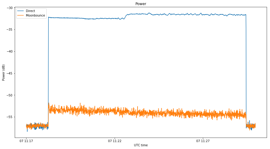
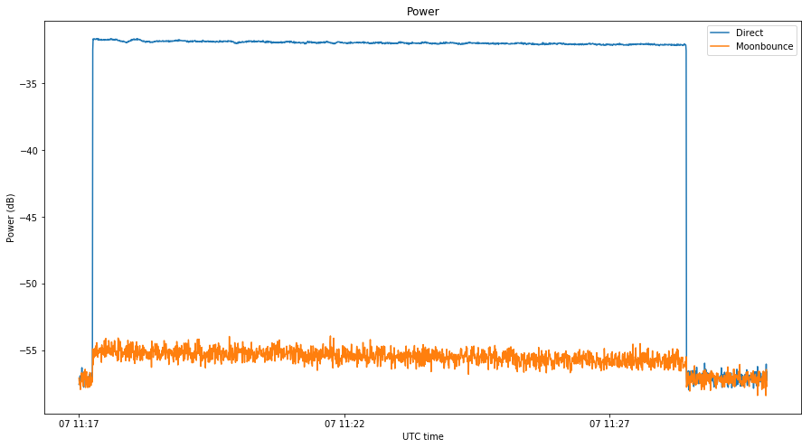
Getting good results in this analysis has not been so easy because the SNR of the reflected signal is low, as the two images above show. The large Doppler spread also makes long coherent integrations impractical. I have spent a lot of time fine tuning the parameters of the correlations, partly because it is not so clear how to obtain good results (the goal is to be able to discern some characteristics of the reflection from the video qualitatively, not to optimize some quantitative parameter), and partly because the computations are lengthy.
I am interested in any other alternative ways of processing the data that yield better or newer results or insight. Although I think that the SNR is not good enough to be able to model the channel well, I am also interested in seeing if the reflected signal can be modelled as a Rayleigh channel, but I think that I still need to understand fully some key concepts about fading channels to attempt this.
Finally, a good research idea would be to try to determine the area of the lunar surface where the reflection happens. I think that my data shows that this area is centred on the point predicted by the specular reflection model, but I have no clue about how large or small this area is. Ideally one would like to determine the energy density of the reflection over the lunar surface. I still haven’t thought much about how to do this, but I think that the profile of Doppler spread can be a good tool. The fact that the correlation peak is not smeared also sets an upper bound for the size of the reflection area (compare the size of one symbol, which is 1200km with the lunar radius, which is 1737km).
As a small remark, after seeing the Doppler spread, I think that decoding the data from the reflected signal is very difficult or impossible. Not only the signal is weak, but also the Doppler spread of 50Hz is quite large in comparison with the symbol rate of 250baud. It would be a real challenge to estimate the phase of the signal and to design a PLL which doesn’t slip.
3 comments