In a previous post I showed how to demodulate the LTE physical uplink shared channel (PUSCH) by using a recording of my phone and some Python code. This is a continuation of that post. Here we will look at the physical uplink control channel (PUCCH) transmissions in that recording, and use a similar approach to demodulate them. All the work is done in a Jupyter notebook, which is linked at the end of the post.
The PUCCH carries control information from the UE to the eNodeB, such as scheduling requests, ACK/NACK for HARQ, and the CQI (channel quality indicator). A PUCCH transmission lasts for one subframe (1 ms) and typically occupies a single 12-subcarrier resource block in each of the two 0.5 ms slots in the subframe (there are more recently introduced PUCCH formats which use more subcarriers).
PUCCH transmissions are allocated to the edges of the uplink bandwidth, so as to leave the centre clear as a contiguous segment to be used for PUSCH. On its first slot, the PUCCH transmission uses some particular resource block. On its second slot it uses the symmetric resource block with respect to the centre frequency. This gives some frequency diversity to the transmissions.
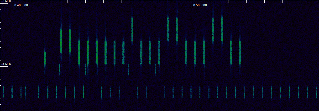
The figure below shows a portion of the waterfall of the LTE uplink recording that we will be using (the link to the recording is included in the previous post). It corresponds to a 10MHz-wide cell in the B20 band. The PUCCH transmissions are the narrow bursts. The wider stronger bursts are PUSCH.
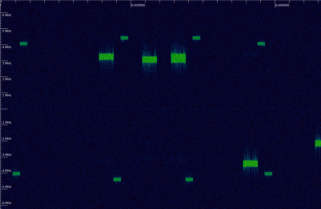
This illustrates that the PUCCH subframes are allocated to the edges of the cell, and how each subframe jumps to the symmetric resource block on its second slot.
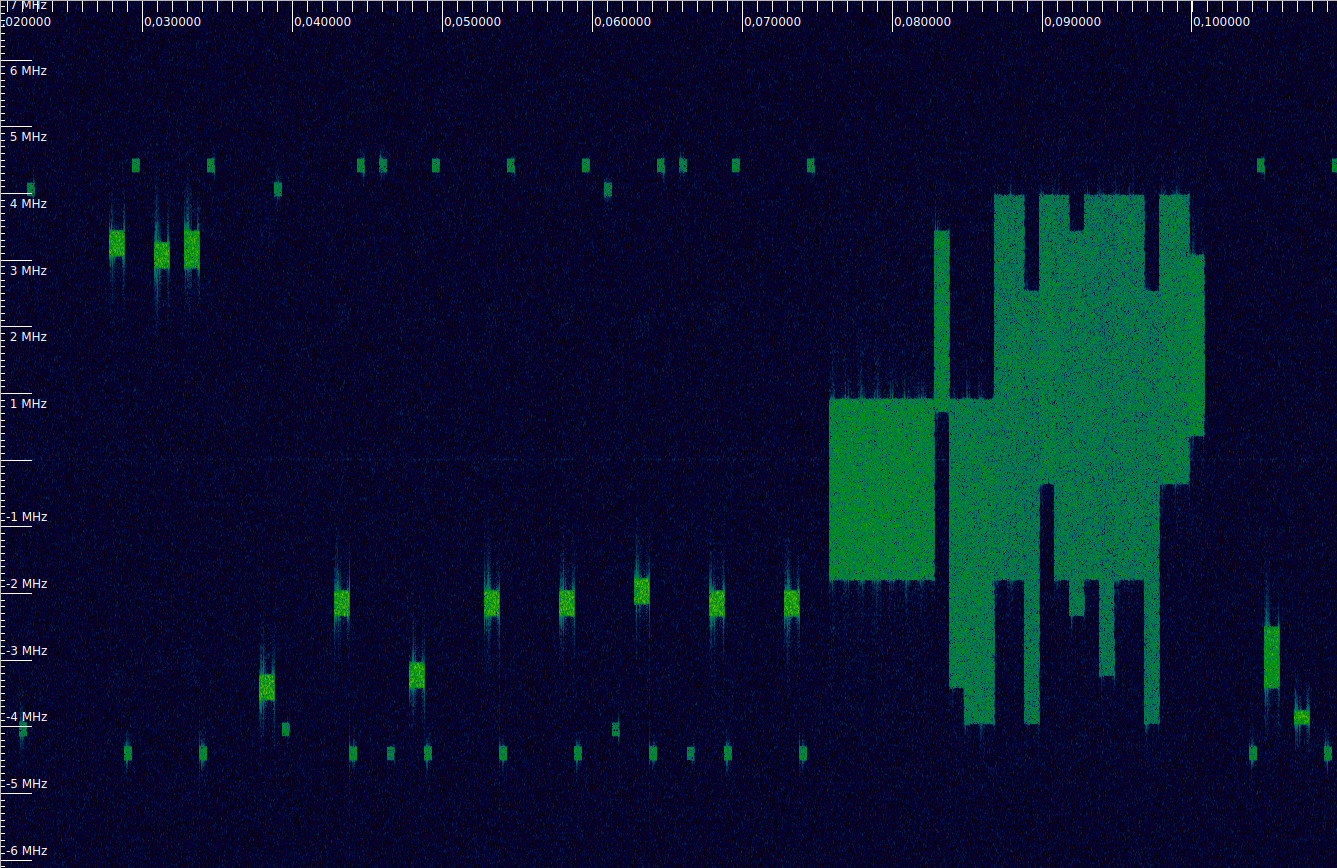
If we zoom out in time we can also see another important aspect. Typically, an UE does not transmit PUSCH and PUCCH simultaneously. Recent additions to the standard allow simultaneous PUSCH and PUCCH transmissions, but these are harder to amplify without distortion, due to the higher peak-to-average power ratio of the resulting waveform. Here we can see that during the long PUSCH transmission between 0.075 and 0.1 seconds in the recording (part of which we analysed in the previous post) there are no PUCCH transmissions.
Synchronization
For time synchronization, I first attempted to use the “poor man’s Schmidl & Cox” method that I presented in the previous post. However, this doesn’t work here. The figure below shows the correlation we obtain with this method. We would expect to see peaks corresponding to the starts of the cyclic prefix of each symbol. However, we don’t see that. We can see that the correlation is large as soon as both \(x(t)\) and \(x(t + T_u)\) are inside the first slot of the PUCCH transmission. Then the correlation drops down when \(x(t + T_u)\) crosses to the second slot (which is at a completely different frequency) while \(x(t)\) is still in the first slot. Finally, the correlation becomes large again when \(x(t)\) crosses to the second slot. The plot doesn’t show a clear indication of the start of each symbol.
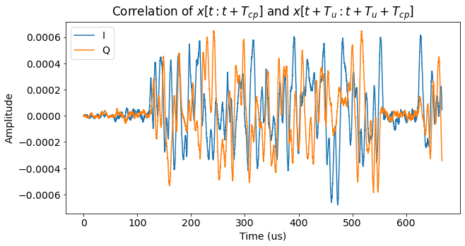
The reason why this technique doesn’t work is essentially that the PUCCH is too narrow. Its bandwidth is 180 kHz, while the reciprocal of the cyclic prefix duration \(T_{cp}\) is 213.33 kHz (or 192 kHz for the cyclic prefix of the first symbol, which is slightly longer). This means that, forgetting about the fact that the PUCCH transmission is not at baseband (which doesn’t matter, because the carrier frequency is cancelled in the correlation), the time-domain PUCCH waveform is more or less constant in every interval of length \(T_{cp}\). This causes the correlation to be large regardless of whether \(t\) is aligned to the start of the cyclic prefix or not.
This reasoning shows that the poor man’s Schmidl & Cox method will only work well when the bandwidth of the OFDM transmission is much larger than \(1/T_{cp}\).
If we want to achieve time synchronization using only the PUCCH transmissions, then performing power detection of the start and end of the two slots of each transmission seems a good approach. We can take advantage of the fact that there are often many PUCCH transmissions, so if the SNR is not too good we can measure several of them and do an average.
In this case, since I had already done synchronization using the PUSCH in the previous post, I have used the estimates from that post for symbol time and carrier frequency offset.
OFDM demodulation
Looking at the waterfall, we can see that in this recording the PUCCH transmissions only happen in 4 different resource blocks. Using the same numbering for the OFDM subcarriers as in the previous post, these use subcarriers 725-736, 749-760, 1289-1300, and 1313-1324. They correspond to the 23rd and 25th resource blocks to the left and right of DC. Since a 10 MHZ LTE cell is 50 resource blocks wide, we see that the resource blocks used by our PUCCH transmissions are numbers 0, 2, 47, and 49 (where we number the 50 resource blocks from 0 to 49).
OFDM demodulation is performed in the same way as in the previous code. The PUCCH doesn’t use the DFT SC-FDMA precoding that is used in the PUSCH data symbols. For each symbol, we do power detection to determine in which of the 4 possible resource blocks the symbol is transmitted, and store only the OFDM symbols from the 12 subcarriers of that resource block.
We demodulate all the recording length, which is ~0.9 seconds. In order to detect when the PUCCH transmissions happen, we compute the average power in each slot and perform a power detection. The plot below shows the result of this power detection, as well as the threshold that I have used to decide which slots really have PUCCH.
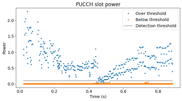
I have needed to adjust the threshold carefully, because in the middle of the recording the power of the PUCCH transmissions drops significantly. I think this may be my phone doing some sort of transmit power control. However, the attenuation between the phone and the USRP B205mini which I used to record was by no means well controlled. The recording was done by simply holding the phone close to the B205mini without any antenna attached. Therefore, the power measurements should be interpreted carefully.
There are also some slots that contain leakage from PUSCH transmissions using resource block 3, which is adjacent to one of the PUCCH resource blocks. I have taken care to avoid detecting these as PUCCH transmissions. The waterfall below shows the lower edge of the cell at ~0.5 seconds in the recording. We can see the leakage from the PUSCH transmissions and also the sudden drop in transmit power, which seems to affect both PUSCH and PUCCH. Also note that generally PUCCH is transmitted with less power than PUSCH, which makes sense, since it carriers less data.
We have detected a total of 178 PUCCH transmissions in the recording. The constellations of the OFDM symbols corresponding to the first 4 of them are shown below. The slots in this table are numbered relative to the first slot of the first PUCCH transmission in the recording. For instance, the second transmission starts 7 ms after the start of the first transmission, so it occupies slots 14 and 15.
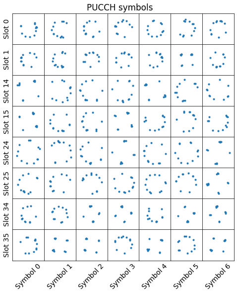
From these constellation plots we see that the PUCCH OFDM symbols are complex number of modulus one. The constellation of some of the symbols looks like a QPSK constellation, while other symbols have their constellation spread around the unit circle. We will see why this happens when explain the structure of the PUCCH symbols below.
PUCCH waveform structure
While doing this work, besides the 3GPP TS 36.211 document, I have also found quite useful the book LTE-Advanced – A Practical Systems Approach to Understanding 3GPP LTE Releases 10 and 11 Radio Access Technologies, by Sassan Ahmadi. In comparison to TS 36.211, this book is easier to read, because it contains explanations about what is the intention or background of the different aspects of the physical layer, and how they relate to each other. In this respect, TS 36.211 really contains all the information, but often it’s necessary to keep jumping between several sections (or even moving to other documents about the higher protocol layers), and there are no explanations about why things are done in a particular way. I think that the LTE-Advanced book doesn’t attempt to have all the formulas and level of detail of TS 36.211, but there is enough detail to find most stuff, and jumping from this book to TS 36.211 to complete what’s missing is not difficult.
The PUCCH symbols are constructed using a base sequence \(r_u(n)\), \(n=0,\ldots,11\). The base sequences are indexed with the group number \(u\), which is an integer between 0 and 29. The sequence has the form\[r_u(n) = e^{i\varphi_u(n)\pi/4},\]where the possible values of \(\varphi_u(n)\) are \(\pm 1\) and \(\pm 3\). The functions \(\varphi_u\) are listed, for each \(u\), in Table 5.5.1.2-1 in TS 36.211. This means that each of the sequences \(r_u\) is a sequence of 12 QPSK symbols of the form \((\pm 1 \pm i)/\sqrt{2}\).
These base sequences are intended to play the same role as Zadoff-Chu sequences (see the previous post) and to have similar properties. The reason why these QPSK sequences are used for PUCCH instead of Zadoff-Chu sequences is because Zadoff-Chu sequences don’t work too well for 12 subcarriers, because extending a length 11 Zadoff-Chu sequence to a sequence of length 12 loses some of its properties, and also there are not 30 Zadoff-Chu sequences of length 11 to choose from. In fact, Zadoff-Chu sequences are only used for transmissions that use 3 resource blocks (36 subcarriers) or more. For narrower transmissions, computer optimized sequences like these base sequences are used.
Similarly to the PUSCH DMRS, the base sequence for PUCCH is always used with a cyclic shift as\[r_u^\alpha(n) = e^{i\alpha n} r_u(n),\]where the shift \(\alpha\) is of the form \(\pi k/6\), for \(k = 0,1,\ldots, 11\). The value of \(\alpha\) changes for each symbol following a pseudorandom sequence. Note that when \(k\) is divisible by 3, then \(r_u^\alpha(n)\) is still a sequence of QPSK symbols, but in general the constellation of \(r_u^\alpha(n)\) covers more than four points of the unit circle.
There are several formats for PUCCH transmissions. Here we will only deal with formats 1/1a/1b and 2/2a/2b, as they are the most common and the only ones that appear in the recording.
Format 1/1a/1b
Format 1/1a/1b carries a single value \(d(0)\) in all the PUCCH transmission. For format 1, \(d(0)\) always equals 1, and information is transmitted by the presence or absence of such a transmission. This format is used to send a scheduling request from the UE. For format 1a, \(d(0)\) is a BPSK symbol. The value \(d(0)=1\) corresponds to a logical 0, which means a HARQ NACK, and \(d(0)=-1\) corresponds to a logical 1, which means a HARQ ACK. Format 1b carries a QPSK symbol using the values \(\pm 1\) and \(\pm i\), to represent two bits of HARCK ACK/NACK. This is used for downlink spatial multiplexing, which I believe doesn’t happen in this recording.
The three symbols in the middle of each format 1/1a/1b PUCCH slot are used for DMRS (demodulation reference signal), while the first two and last two are data. The DMRS symbols are defined by\[w(m)r^\alpha_u(n),\quad m = 0, 1, 2,\ n = 0, 1, \ldots, 11.\]Here \(m\) indicates the symbol number, and \(n\) is the subcarrier number. There are three possible choices for the spreading sequence \(w(m)\). It can be either \(1, 1, 1\), or \(1, e^{2\pi i/3}, -e^{2\pi i/3}\), or \(1, e^{-2\pi i/3}, e^{2\pi i/3}\) (note that these are the Fourier basis of dimension 3). For each slot, one of the three possible sequences is chosen pseudorandomly.
The data symbols are formed as\[S(n_s)w(m)d(0)r^\alpha_u(n),\quad m=0,1,2,3,\ n = 0, 1, \ldots, 11.\]Here \(m\) indexes the four data symbols in each slot and \(n_s\) indicates the slot number. There are three possible choices for \(w(m)\), corresponding to the three choices of \(w(m)\) for the DMRS. In each slot, the same corresponding choice is used for the data \(w(m)\) and for the DMRS \(w(m)\). The three choices for the data \(w(m)\) sequence are 1,1,1,1, or 1, -1, 1, -1, or 1, -1, -1, 1 (note that these are extracted from a Hadamard basis of dimension 4). The value of \(S(n_s)\) is either \(1\) or \(i\).
Format 2/2a/2b
Formats 2/2a/2b are used to send CQI (channel quality indicator) data, so they need to send much more data than format 1/1a/1b. This is mainly accomplished by sending a different value in each of the symbols (recall that the 8 data symbols of a format 1/1a/1b transmission carry the same value \(d(0)\)). For these formats, the second and second to last symbol in each slot are DMRS, while the remaining 5 symbols in each slot (the first, the three in the middle, and the last) carry data. This gives us 10 data symbols \(d(0),d(1),\ldots,d(9)\) in the transmission (which lasts 2 slots). These data symbols are taken from a QPSK constellation formed by the points \((\pm 1 \pm i)/\sqrt{2}\).
The DMRS symbols are defined by\[z(m)r^\alpha_u(n),\quad m=0,1,\ n = 0,1, \ldots, 11.\]Here \(m\) indexes the two DMRS symbols in each slot and is only used in formats 2a and 2b to squeeze in an 11-th data symbol by setting \(z(0) = 1\) and \(z(1) = d(10)\). In contrast to the remaining symbols, \(d(10)\) uses the same constellations as format 1a/1b. For format 2a \(d(10)\) carries a BPSK symbol encoded as \(\pm 1\), and for format 2b, \(d(10)\) carries a QPSK symbol encoded as \(\pm 1\) and \(\pm i\). For format 2, there is no 11-th data symbol and \(z(0) = z(1) = 1\).
The data symbols are modulated as\[d(m)r^\alpha_u(n),\quad m=0, 1, \ldots, 9,\ n = 0, 1, \ldots, 11,\]where \(m\) indexes the 10 data symbols in the PUCCH subframe.
Handling the base sequence
The first step to process the PUCCH symbols is to find the base sequence group \(u\) and to determine, for each symbol, the cyclic shift parameter \(\alpha\). The method we use to do this was introduced in the previous post. To find the group, we take a PUCCH symbol and multiply it with the complex conjugate of each of the 30 possible base sequences. Then we take the Fourier transform of this product. For the matching sequence, this Fourier transform will show a peak corresponding to the cyclic shift \(\alpha\) used in this symbol. For the remaining base sequences, the power will be randomly spread over all the Fourier bins.
This works because regardless of the PUCCH format the product for the matching base sequence will be of the form \(\lambda e^{i\alpha n}\) for some complex number \(\lambda\) (whose amplitude will in general not be one unless the amplitude of the signal has already been equalized). Therefore, the Fourier transform is \(\lambda\) times a Dirac delta whose position corresponds to the value of \(\alpha\).
The results of this calculation are shown in the figure below.
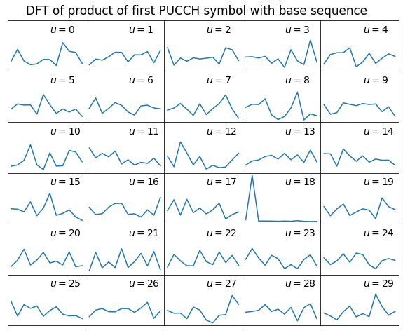
We can see that the matching base sequence has \(u = 18\). This is the same group that was used for the PUSCH transmissions that we analysed in the previous post. This is not a coincidence. Unless some features such as group hopping or virtual cell identity are enabled, the base sequence used both for PUSCH and PUCCH is simply the physical cell ID (PCI) modulo 30. The LTE discovery app on my phone shows a PCI of 378 when connected to this cell, which makes sense, as 378 modulo 30 is 18.
Now that we have determined the base sequence to use, we need to determine the value of \(\alpha\) for each symbol. The same approach is used. The symbol is multiplied with the complex conjugate of the base sequence \(r_u(n)\) for the correct \(u = 18\), and the Fourier transform is calculated. The bin where the maximum amplitude is attained gives the value of \(\alpha\).
Once the values of \(\alpha\) for all the symbols have been computed, each of the symbols can be multiplied by the complex conjugate of the corresponding shifted base sequence \(r^\alpha_u(n)\) in order to wipe the sequence off. What we obtain in the 12 subcarriers of each symbol is the same complex number, except for the fact that the channel impulse response affects each of the subcarriers differently. We will use this property for equalization, in order to correct the symbol time offset.
Symbol inversion
At this point we have to perform a step for which I’ve had a rather hard time finding any mention or justification in the LTE documentation. It turns out that we need to multiply every other symbol by -1 in order to flip its phase by 180 degrees. I even asked about this on Twitter, to see if someone could give me an idea, but I got nowhere.
Something like this already appeared in the previous post, as I found that I needed to multiply by -1 the DMRS in every other slot. Taking into account that the number of symbols in a slot is odd (there are 7 symbols in a slot) and that the DMRS occupies the same position in all the slots (the middle symbol), if we multiply every other symbol by -1, then the effect is that every other DMRS will be multiplied by -1.
In fact, since I wasn’t looking at the PUSCH data besides plotting the QPSK constellation, a 180 degree flip in the data symbols wouldn’t have been visible. By looking at the DMRS alone, I wasn’t able to tell whether these flips should affect the DMRS only, or every other slot as a whole, or every other symbol. Now that I’m looking at the PUCCH, these differences become visible.
The reason why I came to the conclusion that we need this symbol inversion can be seen by looking at the DMRS for the format 1/1a/1b PUCCH. If we take one of these PUCCH transmissions such that the spreading code \(w(m)\) is not 1, 1, 1, then the phases of the 3 DMRS symbols should be spaced 120 degrees apart (or in other words, give the vertices of an equilateral triangle when we plot them on a constellation diagram). This is simply because \(w(m)\) must be either \(1, e^{2\pi i/3}, e^{-2\pi i/3}\) or \(1, e^{-2\pi i/3}, e^{2\pi i/3}\), and the spacing of the phases of the three symbols (or the shape they draw on a constellation diagram) won’t change if we multiply the whole signal by a complex number \(\lambda\) (which is the situation before we have equalized the phase offset and amplitude of the signal).
However, if we don’t perform the symbol inversion, then we find that the 3 DMRS symbols are spaced only 60 degrees apart (such as \(1, e^{\pi i/3}, e^{2\pi i/3}\)). Note that if we have such a sequence and we multiply by -1 either the symbol in the middle, or the two symbols in the ends, then we obtain three points which are 120 degrees apart as they should.
It is interesting that, without trying to interpret the values of the QPSK symbols in PUCCH format 2/2a/2b, this is the only place where this kind of symbol inversion can be detected or investigated. In the data symbols of format 1/1a/1b, the symbol inversion can be mistaken with the \(w(m)\) sequence that alternates signs, and the format 2/2a/2b DMRS symbols are located in symbols 1 and 5 (counting from 0 to 6) in each slot, so they have the same “parity” and get the same inversion.
I found almost by chance the clue that led me to understand this issue, and only after having nearly finished writing this post. It has to do with the way that the LTE uplink subcarriers are shifted in frequency by half a subcarrier spacing to avoid having a subcarrier at DC. I this Keysight documentation, they explain this fact and use the term “phase reset”. The way I had dealt with this property was simply to shift by signal by 7.5 kHz. However, this is not exactly what needs to be done.
If we look attentively at the formula in Section 5.6 of TS 36.211 that describes how the continuous-time uplink baseband signal is generated,\[s_l^{(p)}(t) = \sum_{k=-\lfloor N_{RB}^{UL}N_{sc}^{RB}/2 \rfloor}^{\lceil N_{RB}^{UL}N_{sc}^{RB}/2 \rceil -1} a_{k^{(-)},l}^{(p)}\cdot e^{i2\pi (k+1/2)\Delta f(t-N_{cp,l}T_s)},\]valid for \(0\leq t\leq (N_{cp,l}+N)T_s\), we readily see the 7.5 kHz shift as the \(1/2\) term in the exponential. However, note that for \(t = N_{cp,l}T_s\), which corresponds to the start of the useful symbol, the value of the exponential is just one. This is what Keysight mean by phase reset. The whole uplink waveform is constructed by forming these time-domain symbols \(s_l^{(p)}(t)\) for \(0\leq t\leq (N_{cp,l}+N)T_s\) and translating each of them in time to its appropriate location. Therefore, for each symbol the phase of the exponential is zero at the start of the useful symbol.
Compare this with a frequency shift of \(\Delta f/2\), which is given by \(e^{\pi i \Delta f t}\). The phase of the exponential is not zero at the start of each symbol. If there was no cyclic prefix, so that the symbol duration is exactly \(1/\Delta f\), then the phase of the exponential would alternate between 0 and 180 degrees every other symbol. This is where the symbol inversion I need to do ultimately comes from.
However, due to the cyclic prefix, the phase of the exponential \(e^{\pi i \Delta f t}\) advances somewhat more than 180 degrees per symbol. It advances 194 degrees during the first symbol in each slot (which has a slightly longer cyclic prefix), and 192.7 degrees during each of the remaining symbols. In total, it advances exactly 1350 degrees in each slot, which reduced modulo 360 degrees is -90 degrees. This means that we have an apparent extra frequency offset of -90 degrees every 0.5 ms, which is -500 Hz. This offset will be absorbed by our carrier frequency offset estimation. The phase difference due to the duration difference between the first and the remaining cyclic prefixes is small enough that most likely we will not notice.
In hindsight, it is clear that one should not shift the uplink waveform by 7.5 kHz before OFDM demodulation, but rather take into account properly this phase reset and perform the frequency shift during the OFDM demodulation of each symbol. However, here I have tried to explain why if one ignores the phase resets and does the 7.5 kHz shift to the whole waveform (which is what I have in the Jupyter notebooks, since I have not corrected this), then the results are almost perfect except for the fact that the phase of every other symbol needs to be flipped.
Equalization
As in the previous post, we assume that there is no multipath, so that the channel impulse is a single Dirac delta. At this point we will equalize the signal amplitude (which as we have seen above varies quite a bit), and the symbol time offset.
To estimate the signal amplitude we compute the average power in each slot. The next figure shows the amplitude measurements in dB units. Each slot is coloured according to whether it is transmitted in one of the resource blocks near the lower frequency edge of the cell, or in one of the resource blocks near the upper frequency edge of the cell.
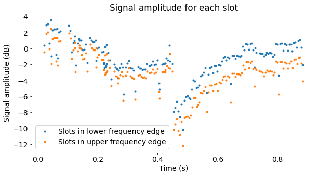
We can see that the transmissions in the upper edge have slightly less power than those in the lower edge. This is not so surprising, as there are about 9 MHz of frequency difference between the two edges. The difference may be caused by the propagation path between the phone and the USRP, by the frequency response of the USRP, by the phone itself, or probably by a combination of all these.
Since we have wiped off the base sequence in each PUCCH symbol, the phase versus frequency of the 12 subcarriers of each symbol follows a slope that indicates the symbol time offset. To estimate the offset, we work with each symbol separately. We compute the average of the 12 subcarriers to obtain a phase reference for that symbol, and use that phase reference to rotate all the subcarriers of that symbol so that they are close to zero. Then we fit a polynomial of degree one to the phases of the 12 subcarriers. The leading term of this polynomial gives the delay estimate for this symbol. The estimates of the 7 symbols in each slot are averaged together so as to produce one estimate per slot.
The figure below shows the symbol time offset estimates. We can see that the offset grows roughly linearly with time. This is caused by a sampling frequency offset (which is slightly above 1 ppm, since in one second the offset increases by slightly more than 1 us).
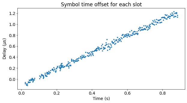
The final offset of approximately 1 us is small in comparison with the symbol duration, and even with the cyclic prefix duration. However, if the offset grew larger because the recording was longer or the sampling frequency offset was larger, then we might want to correct it in our OFDM demodulation to avoid inter-symbol interference.
Once we have the amplitude and symbol time offset estimates, we can apply them to our PUCCH symbols. After doing this, in each subcarrier we obtain a complex number of modulus close to one, and all the 12 subcarriers in the same symbol have very similar values. However, the phase of these may still be anything, since the phase offset hasn’t been equalized yet. To do this, we first need to identify the format of each PUCCH transmission in order to select the correct DMRS symbols.
Identifying the PUCCH formats
To interpret the symbols in the PUCCH transmissions correctly, we need to classify them according to their format. We could probably do this just by looking at the resource blocks they use, since format 2/2a/2b transmissions are allocated to the outermost resource blocks, and format 1/1a/1b transmissions are allocated closer to the centre, but the sizes of these allocations depend on the configuration parameters of the cell.
Distinguishing format 1/1a/1b from format 2/2a/2b can be a bit tricky due to all the possible choices for the spreading sequences \(w(m)\). However, a singular feature of format 2/2a/2b is that its data symbols (which are QPSK) are offset by odd multiples of 45 degrees with respect to its DMRS symbols. In contrast, in format 1/1a/1b it is not possible to obtain a difference which is an odd multiple of 45 degrees between any of the symbols, because the possible symbols are \(\pm 1\), \(\pm i\), and \(e^{\pm 2\pi i/3}\).
Therefore, we do the following. We take the 7 symbols in each slot and use the second symbol as a phase reference, rotating all the 7 symbols by the opposite of the phase of the second symbol (for format 2/2a/2b this symbol should be 1, so it really is a proper phase reference). Now we take all the symbols except the second and second to last (so if this is a format 2/2a/2b transmission, we are taking the QPSK data symbols), and compute their 4-th power. Due to how the QPSK constellation is defined as the points \((\pm 1 \pm i)/\sqrt{2}\), if this is a format 2/2a/2b transmission, we expect to get something quite close to -1 for all these symbols. For a format 1/1a/1b transmission we get something which is away from -1. So we compute the RMS distance of these 5 symbols from -1 and decide whether the format is 1/1a/1b or 2/2a/2b depending on whether the distance is large or small.
The plot below shows the values of the RMS distance metric and the threshold I have chosen. We see that most of the transmissions are format 2/2a/2b.

This shows the format for each PUCCH subframe according to our detection.

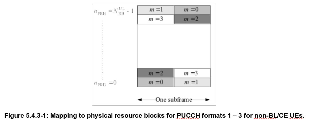
Additionally, we can look at the resource blocks used by each of the PUCCH formats. Numbering the resource blocks from 0 to 49, we see that PUCCH format 1/1a/1b transmissions use RB1-RB48, RB48-RB1, or RB49-RB0, while PUCCH format 2/2a/2b transmissions always use RB0-RB49.
Comparing this with the figure of PUCCH resource block allocations in TS 36.211, we see that format 2/2a/2b transmissions are using \(m = 0\), while format 1/1a/1b transmissions are using \(m = 1, 2, 3\). This makes sense, because format 2/2a/2b transmissions are allocated to lower indices \(m\).
PUCCH format 2/2a
We now take the transmissions that have been detected as format 2/2a/2b in the previous step and use the second symbol in each slot as a phase reference. We can directly plot the resulting constellation, where each subcarrier and symbol is plotted as a different point (recall that the 12 subcarriers in each symbol really have the same data).
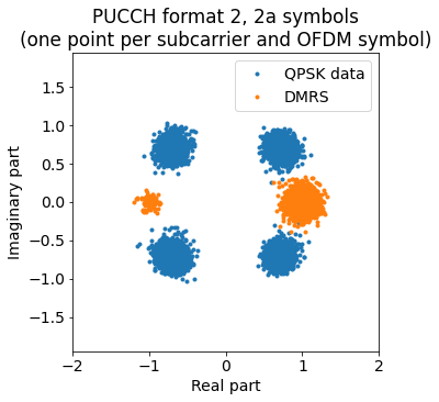
As expected, the data symbols are points from the constellation \((\pm 1 \pm i)/\sqrt{2}\). Most of the DMRS symbols correspond to the constellation point 1, but there are a few of them that correspond to the constellation point -1. These are given by the second DMRS symbol in each slot of those format 2a transmissions for which \(d(10) = -1\). It seems that there are no format 2b transmissions, but we wouldn’t be able to spot them unless they have \(d(10) = \pm i\), for otherwise they would look the same as a format 2a transmission.
PUCCH format 1/1a
For PUCCH format 1/1a/1b we need to do more work than for format 2/2a/2b, because we need to handle the spreading code \(w(m)\). First we need to detect what spreading code has been used. For the DMRS, we perform an FFT of the three symbols. The location of the peak will tell us whether \(w(m)\) is the sequence \(1, 1, 1\) or \(1, e^{2\pi i/3}, e^{-2\pi i/3}\) or \(1, e^{-2\pi i/3}, e^{2\pi i/3}\). Once that we know the correct sequence, we can wipe it off, average the three DMRS symbols together, and use that as a phase reference.
For the data symbols, we can compute the correlations with the three possible sequences 1, 1, 1, 1, and 1, -1, 1, -1, and 1, -1, -1, 1, and choose the one with largest amplitude. Alternatively, we could use the fact that we know that the DMRS and data \(w(m)\) sequences should match, so for instance if \(1, e^{2\pi i/3}, e^{-2\pi i/3}\) was used for the DMRS, then the data symbols should use 1, -1, 1, -1. However, I’ve chosen to detect the sequence of the data symbols independently, and then use this fact as a cross-check.
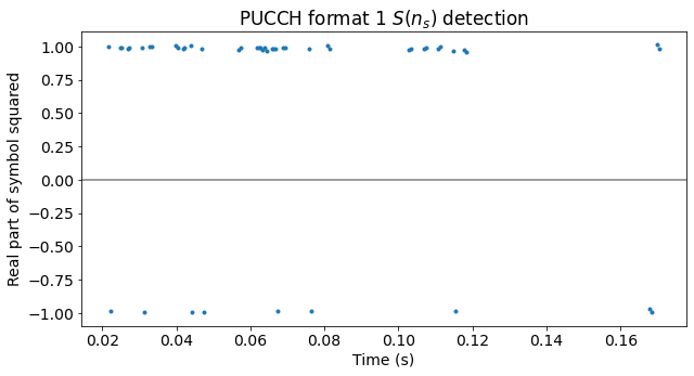
The next step is to determine \(S(n_s)\). Here we use the fact that we don’t expect to see format 1b transmissions, so the values of \(d(0)\) are real. Then we can average the four data symbols in each slot (after wiping off \(w(m)\)), compute the square and look at the real part. If the real part is positive, then \(S(n_s) = 1\), and if the real part is negative, then \(S(n_s) = i\). For format 1b transmissions we would have more difficulties, because unless we are able to compute \(S(n_s)\) independently, we could have trouble deciding whether the value of \(S(n_s)\) is \(1\) or \(i\) just by looking at the product \(S(n_s)d(0)\), as in this case \(d(0)\) can be \(\pm 1\) or \(\pm i\).
The next figure shows the real parts of the squares of the symbols, which we use to detect when \(S(n_s) = i\). We see that this only happens a few times.
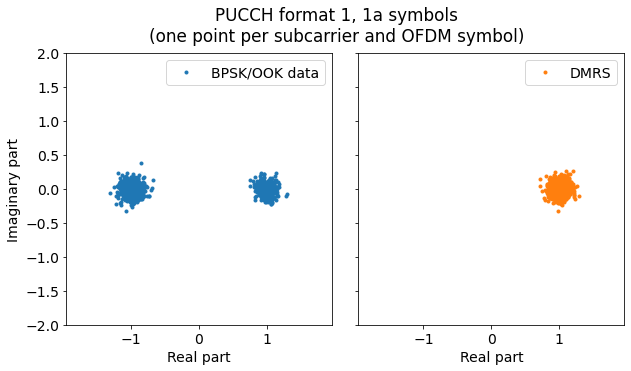
After wiping off the sequences \(w(m)\) and \(S(n_s)\), we can now plot the constellations for the data symbols and the DMRS symbols. The data symbols have a BPSK constellation, while the DMRS symbols are all +1.
We can now extract the data \(d(0)\) from each PUCCH format 1/1a subframe. These are shown below.
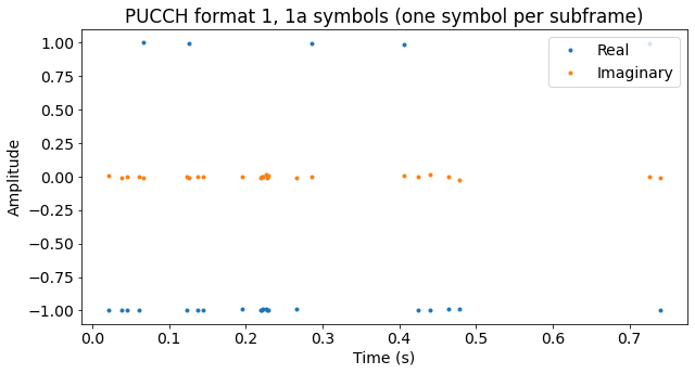
Perhaps the next figure is more clear. It shows the symbols equally spaced in time, regardless of their actual transmission time.
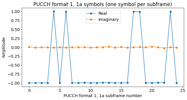
Recall that for format 1 the symbol \(d(0)\) equals 1, and the transmission is a scheduling request. For format 1a, the symbol \(d(0)\) equals 1 to transmit the bit 0, indicating a HARQ NACK, while the symbol \(d(0)\) equals -1 to transmit the bit 1, indicating a HARQ ACK. We see that most of the transmissions are format 1a carrying a HARQ ACK. I guess this makes sense, given that my phone should have had a relatively good signal from the eNodeB.
Code and data
The Python code used for the calculations and figures in the post can be found in this Jupyter notebook. The IQ recording is in this location.
Update 2023-09-27: I have updated the Jupyter notebook to handle the 7.5 kHz uplink subcarrier offset correctly, as indicated in the “Symbol inversion” section. By doing this, the sign change in every other symbol does not appear. For more details see this comment in the previous post.
3 comments