Studying Es’hail 2 Doppler

Es’hail 2, the first geostationary satellite carrying an Amateur radio payload, was launched on November 15. I wrote a post studying the launch and geostationary transfer orbit, and I expected to track Es’hail 2’s manoeuvres by following the NORAD TLEs. However, for reasons not completely known, no NORAD TLEs were published during the first two weeks after launch.

On November 23, people found Es’hail 2 around the 24ºE geostationary orbital slot by receiving its Ku-band beacons at 10706MHz and 11205MHz. On November 27, NORAD TLEs started being published, confirming the position of Es’hail 2 around 24ºE. Since then, it has remained in this slot. Apparently, this is the slot that will be used for in-orbit test before moving the satellite to its operational slot on 25.5ºE or 26ºE.

Since November 27, I have been monitoring the frequency of the 10706MHz beacon to measure the Doppler. A geostationary satellite is never in a fixed location as seen from the Earth. It moves slightly due to imperfections in its orbit and orbital perturbations. This movement is detectable as a small amount of Doppler. Here I study the measurements I’ve been doing.

The measuring equipment is a 95cm offset dish from Diesl.es, an Avenger PLL321S-2 Ku-band LNBF, modified to use an external reference, and a LimeSDR. Everything is disciplined to a DF9NP GPSDO. The LimeSDR uses the 10MHz output from the GPSDO (see this post), while the LNBF is fed a 27MHz reference from a DF9NP PLL. From the software side, I’m using WSJT-X in frequency measurement mode, as I detailed in my post about TCXO stability.

The measurements from WSJT-X are read using this Jupyter notebook, which filters out some incorrect measurements and saves them in netCDF4 format for later analysis. The resulting netCDF4 file can be downloaded here.

The analysis of the measurements is done in this Jupyter notebook.  The figure below shows the raw frequency measurements from WSJT-X, expressed as a frequency offset in ppb from the nominal frequency of 10706MHz. We can see that there is a sinusoidal component, which is due to Doppler, and a linearly increasing component, which is probably due to some kind of aging in the on-board clock.

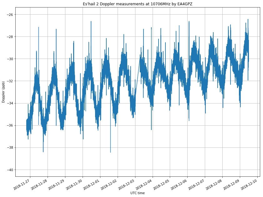
Note that there is a gap in the data in the night between December 3 and December 4, since my measurement system failed.

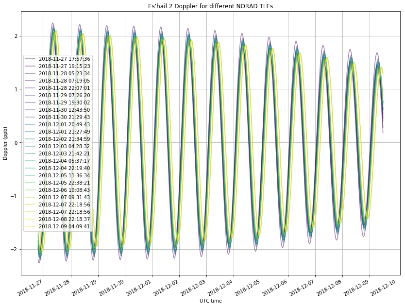
The figure below shows the Doppler calculated using all the TLEs published in Space-Track since November 27. The Doppler is given in ppb. Note that 1ppb corresponds to a speed of about 0.3m/s. The epoch of the TLE is encoded in the colour of the Doppler curve.  We see that the Doppler curves calculated with all the TLEs are very similar. They show a sinusoidal curve, with slightly decreasing amplitude. Also, in the most recent TLEs, the phase of the sinusoid has been delayed slightly (the curve has moved to the right). More on this later.

The calculations of the Doppler predicted by the TLEs have been done using the Skyfield library. I have found a bug in the calculation of the velocity vector of the satellite done by Skyfield. This bug causes incorrect results, which are quite noticeable for the small Dopplers we are dealing with here. Therefore, the Doppler is computed as the time derivative of the distance to the satellite, instead of as the projection of the velocity vector onto the line of sight vector. This calculation gives correct results.

The reference Doppler curve that we will use is obtained by combining all the Space-Track TLEs in the obvious way: the Doppler at a certain epoch is computed by choosing the TLE whose epoch is nearest. This creates discontinuities at the points where we change from one TLE to the next one.

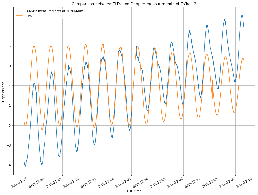
The figure below shows a comparison of my measurements against the reference Doppler curve. I have processed my measurements by averaging in periods of 10 minutes and by subtracting the mean. We see that the sinusoidal components in both curves are approximately the same, but the measurements have a linear drift component that we will now remove.

The figure below shows the difference between both curves, which we will use to measure the linear drift. To perform this estimation, we only select the measurements between 2018-11-28 21:00 and 2018-12-02 20:44:16. This is a time span of exactly 4 sidereal days. Since the period of the sinusoidal component should be very close to one sidereal day, we want to take an integer number of periods so that any periodic components average out. This span was selected because the error in approximating the sinusoidal component is smaller here.

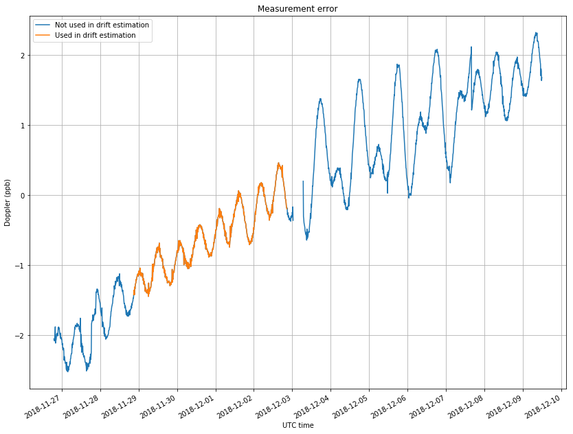
A linear curve is fitted to the orange part of the figure above by using least-squares. The slope of that curve is 4.2e-15 1/s. This amounts to an increase of 0.36ppb per day.

The linear curve we have computed is removed from the measurements. The results are shown in the figure below. We now see that the fit between November 27 and December 3 is very good. This had been already found by Cees Bassa, who analyzed my first days of measurements using his STRF toolkit.

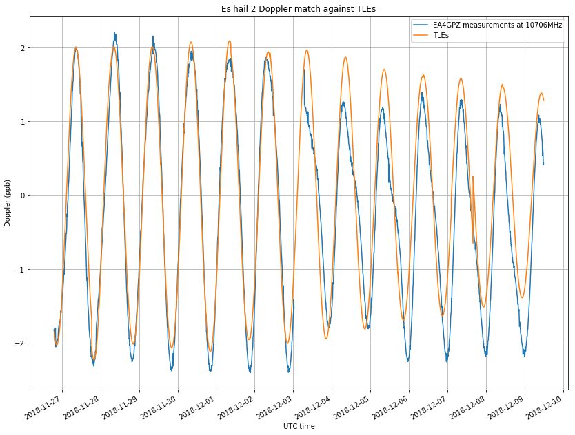
However, after December 3 the fit is not so good. Especially, in December 3, 4 and 5 we have some distortion of the sinusoidal curve after the maximums. I think that this might be caused by manoeuvres of the satellite. Also, note the considerable change of the sinusoidal phase in the reference TLE curve during December 7. I think that Es’hail 2 made some station-keeping manoeuvres between December 3 and 6, and that this only entered the NORAD TLEs on late December 7. Note that the phase of the sinusoid in the measurements changes gradually, so that it doesn’t match the reference TLE during this period. It seems that it matches again towards the end of the plot.

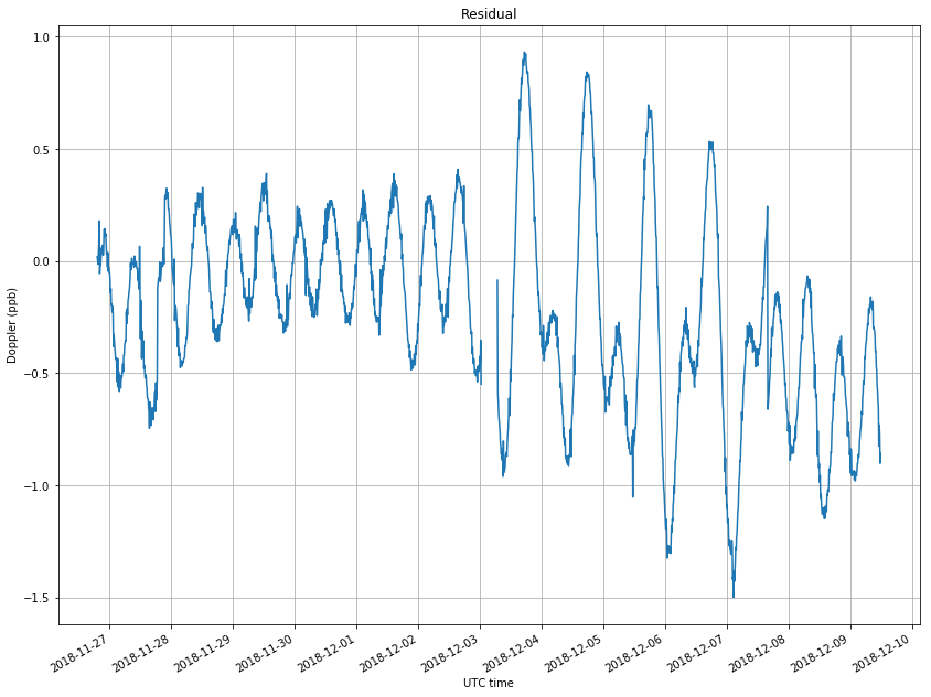
The figure below shows the residual, or the difference between the two curves in the plot above. We see a larger residual between December 3 and 7, as we have explained. Also, the residual of the latest days is no longer centred on zero. This hints at a decrease in the linear frequency drift. Measurements over the next days will confirm if this is the case.

Finally, the figure below shows the position of the satellite, expressed as latitude, longitude and altitude over the ellipsoid. These have also been computed with Skyfield. We see that the latitude and altitude vary sinusoidally, since the inclination and eccentricity of the orbit are not zero exactly. I think this is the main movement that causes the small Doppler we see.

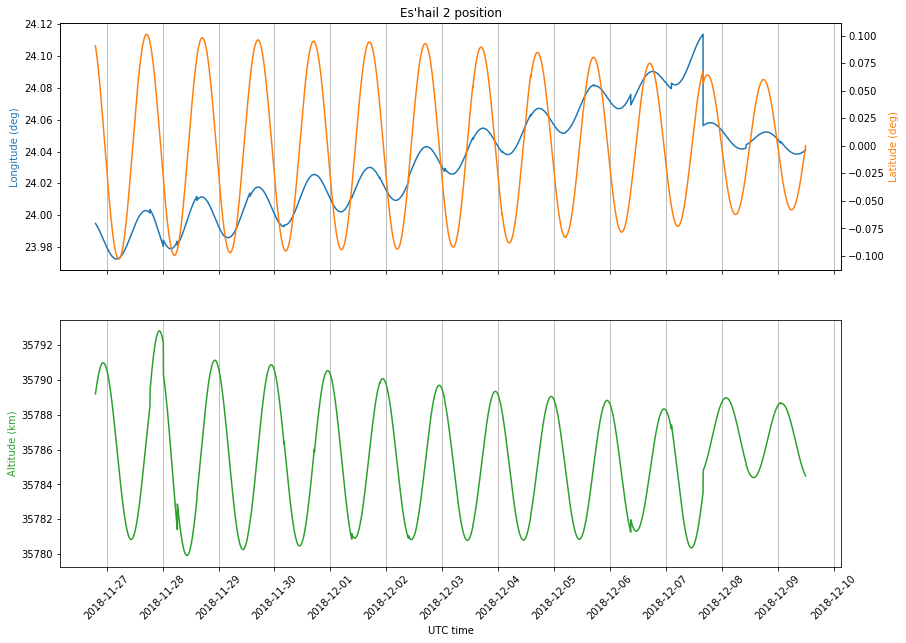
There is also an interesting movement in the longitude. There is a small sinusoidal component, probably due to the nonzero eccentricity, but the main movement is linearly increasing. This is caused by an orbital period which is not exactly one sidereal day. Since the orbital period is slightly smaller than one sidereal day, the satellite keeps drifting east. On December 7 there is a jump in the longitude and the trend after this is decreasing.

This supports my idea of station-keeping manoeuvres between December 3 and 6. The satellite was straying too far east, so small manoeuvres were made to nudge it back towards the west. Of course, the change happened gradually over these days, but NORAD only noticed this change on December 7, thus producing a jump in the TLEs. This movement is what has caused a change of phase in the Doppler curve.

I think I will keep measuring the beacon frequency at least for several days more. It will be interesting if another station makes the same kind of measurements, as this will allow us to remove the transmitter frequency drift completely by subtracting the measurements. Of course, the station would need to be geographically distant from Spain, so as to obtain a good geometry for differencial measurement.