In a previous post I talked about my Doppler measurements of the Es’hail 2 10706MHz beacon. I’ve now been measuring the Doppler for almost a month and this is a follow-up post with the results. This experiment is a continuation of the previous post, so the measurement setup is as described there.
It is worthy to note that, besides the usual satellite movement in its geostationary orbit, which causes the small Doppler seen here, and the station-keeping manoeuvres done sometimes, another interesting thing has happened during the measurement period.
On 2018-12-13 at 8:00 UTC, the antenna where the 10706MHz beacon is transmitted was changed. Before this, it was transmitted on a RHCP beam with global coverage. After the change, the signal was vertically polarized and the coverage was regional. Getting a good coverage map of this beam is tricky, but according to reports I have received from several stations, the signal was as strong as usual in Spain, the UK and some parts of Italy, but very weak or inexistent in Central Europe, Brazil and Mauritius. It is suspected that the beam used was designed to cover the MENA (Middle East and North Africa) region, and that Spain and the UK fell on a sidelobe of the radiation pattern.
At some point on 2018-12-19, the beacon was back on the RCHP global beam, and it has remained like this until now.
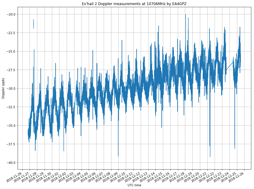
The figure below shows my raw Doppler measurements, in parts-per-billion offset from the nominal 10706MHz frequency. The rest of the post is devoted to the analysis of these measurements.
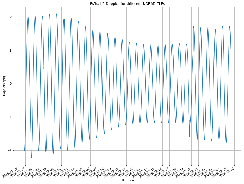
As in the previous post, I have obtained all the TLEs from Space-Track and used them to generate a reference Doppler curve. For each moment in time, I select the TLE whose epoch is nearest, so the Doppler curve has jumps whenever the choice of nearest TLE changes. The jump is more noticeable when suddenly NORAD notices some important change in the orbit, and so the Keplerian parameters change considerably. Note that the Doppler of a geostationary satellite, even if small, is quite sensitive to small changes in the Keplerian parameters. The reference Doppler curve generate from NORAD TLEs can be seen in the figure below.
The figure below shows the comparison of my measurements and the reference Doppler curve. I have averaged my measurements in windows of 10 minutes to reduce the noise. My measurements have a raising trend due to drift in the transmitter. This will be corrected later. Note that there are some gaps in the measurements due to failures in my system or to the observation of the Amateur transponder tests.
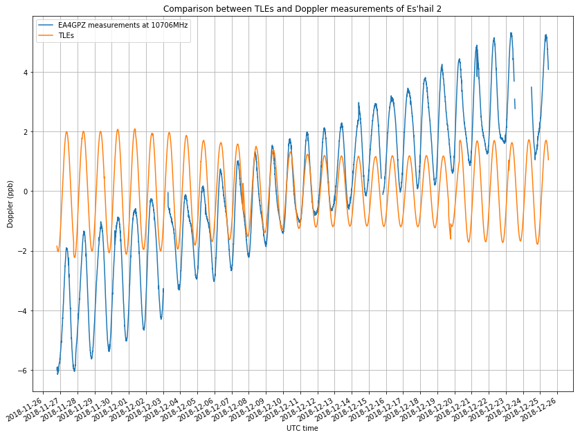
In the previous post I used a linear frequency drift to model the transmitter drift. However, for this longer time frame, we see that the drift is no longer linear, and a quadratic curve is a better match. It would be interesting to observe the drift over the course of several months to see how it evolves.
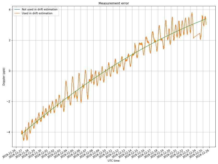
The green curve in the figure above is used as a model for the transmitter drift and subtracted from my measurements. The figure below shows the comparison of the measurements and the NORAD TLEs. Since the Doppler is a sinusoidal curve with a period of one sidereal day, there are two main parameters that we can compare: the amplitude and the phase.
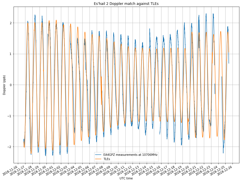
For the amplitude, we see that until December 7 the match is more or less good. It is also good after December 24. However, between these days it seems that the match is not so good, due to an inadequate orbital determination by NORAD. We see that the NORAD Doppler amplitude keeps decreasing until December 20, when it suddenly jumps up again. The measured amplitude also has some decreasing and increasing variations, but is considerably larger than what predicted by NORAD.
The phase in both curves matches pretty well, except in the period between December 3 and 7, when, as remarked in the previous post, a station-keeping manoeuvre happened. Also, there is some amount of phase mismatch between December 15 and 20, but I have no evidence of a manoeuvre made there. Finally, it seems that there is something interesting going on on December 24, but unfortunately I don’t have the whole day worth of data, so I can’t be sure if a manoeuvre was done.
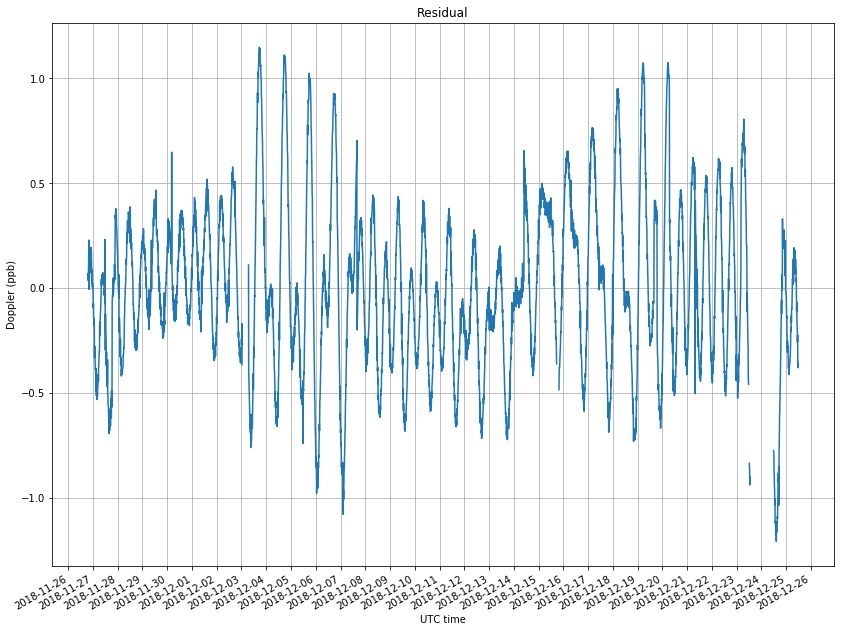
The figure below shows the residuals, which are the difference between the measurements and the NORAD TLEs.
Finally, to give some geometric intuition into this study, it is worth to plot the position of Es’hail 2 according to the NORAD TLEs. This is done in the figure below, using latitude, longitude and altitude coordinates. As the position of a geostationary satellite in this kind of coordinates should not move, in this way we can see the deviations of the orbit from being perfectly geostationary.
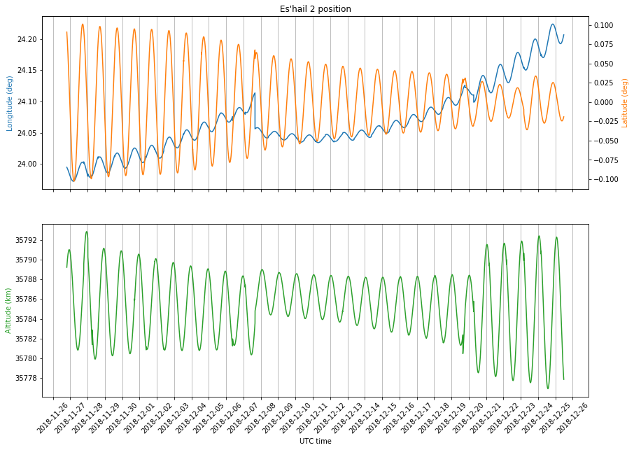
We see that the latitude and altitude trace sinusoidal curves with a period of one sidereal day. It is easy to explain these. The change in latitude is due to a nonzero inclination of the orbit. The amplitude of the latitude oscillations is given by the inclination of the orbit. The phase of these oscillations is directly related to the RAAN of the orbit: the satellite passes through the ascending node whenever the sinusoidal latitude curve increases through zero.
The change in altitude is due to a nonzero eccentricity. The amplitude of the oscillations is given by the eccentricity of the orbit, while the phase is related to the argument of the perigee: the satellite passes through the perigee when the oscillation is at its minimum.
The behaviour of the longitude is more interesting. Disregarding the jump on December 6 due to a station-keeping manoeuvre, there is a quadratically increasing trend and a sinusoidal oscillation with a period of one sidereal day. The sinusoidal movement is also due to the orbital eccentricity. A nonzero eccentricity means that the angular speed of the satellite is not uniform along its orbit (even if its mean motion averages to one rotation per sidereal day). This means that when the satellite is near apogee, it will move slightly slower than average, lagging with respect to Earth’s rotation. When the satellite is near perigee, an opposite effect will cause the satellite to advance with respect to Earth’s rotation. This causes a sinusoidal variation that cancels out over the course of a sidereal day, thus giving no long-term net effect. In orbital dynamics this is known as a periodic effect, in contrast to a secular effect.
The quadratically increasing trend is secular, however: it builds up over the course of sidereal days, moving the satellite more and more to the east. The reason for this movement is the non-spherical gravity of Earth. If you’ve ever seen a geoid map, note that for geostationary satellites situated over Africa, the strength of Earth’s gravity field decreases towards the east. Actually, there is a local maximum at 14.7ºW, near the west coast of Africa and a local minimum at 75.3ºE, just south of India.
A geostationary satellite stationed between these two points will continuously suffer a small force pulling it towards the west, where the Earth’s gravitation field is stronger. The interesting thing is that the reaction of orbiting bodies to perturbing forces is usually opposite from what one would expect. In this case, the westward force opposes the orbital speed, so the orbital speed gets reduced. This means that the orbital period is reduced. Therefore, the satellite tends to orbit faster than the rotation of Earth, and so the net effect is that the satellite seems to move east. Hence without station-keeping manoeuvres, a geostationary satellite between 14.7ºW and 75.3ºE will tend to accelerate and “fall” eastwards towards the minimum at 75.3ºE. Since this movement is (approximately) of constant acceleration, the drift in longitude has a quadratic behaviour.
An interesting aspect of this effect is that perhaps it explains why MELCO has chosen 24ºE as the test slot for Es’hail 2. Maybe they will let it “fall” towards its operational slot at 26ºE over the course of the tests. Indeed, according to the latest TLEs, Es’hail 2 is currently drifting “fast” towards the east, so a correction manoeuvre should be done soon if they want to continue station-keeping at 24ºE.
Finally, let me remark how each of these movements impacts into the Doppler seen by my station. Since the Doppler is the time derivative of the distance to the satellite, the question is how each of these movements affects the distance to the satellite.
First of all, note that the derivative of the distance to the satellite with respect to each of these movements (that is, latitude, longitude and altitude) equals the projection of a unit vector in the direction of the movement (north, east and up, respectively) onto the line of sight vector. With the geometry given by my station (which is the typical geometry for Western European stations), each of these projections is not too small. Stations with a latitude close to 24ºE, near the equator, or with the satellite near the horizon, would find a decreased “sensitivity” to one of these movements.
Note 2018-12-31: I’ve noticed I made a mistake while thinking about the geometry in my head. Actually, the “sensitivity” to changes in altitude is very high (the projection is close to one) regardless of the location of the groundstation. The reason is that since the Earth’s radius is much smaller than the geostationary orbital radius, the line of sight vector and the vector joining the centre of the Earth and the satellite make a small angle.
Second, note that the amplitude of the periodic variations in longitude is perhaps 0.01º, so the effect of these variations is swamped by the variations in latitude, which have an amplitude between 0.05º and 0.1º. Thus, we ignore the movement in longitude.
Now, a movement of 0.1º at geostationary orbit corresponds to approximately 74km. This can be directly compared with the variations in altitude, which have an amplitude of about 5km. Therefore, in the case of Es’hail 2, the major contribution to changes in the distance to the satellite is the movement in latitude, caused by a nonzero inclination.
However, near the end of the time span under study it seems that the amplitude of the latitude variations decreases considerably, while the amplitude of the altitude variations is large. Thus, in this moment, the altitude variations might dominate and the periodic variations in latitude might play a significant role.
The Jupyter notebooks used in this post are fmt.ipynb, to convert the data recorded by WSJT-X to NetCDF4 format, and Doppler analysis.ipynb. The raw Doppler data in in ppb.nc.
Very interesting!
By any chance is there a role to be played by the nonzero inclination as a navigational mechanism to PURPOSEFULLY “drift” to the announced operational slot? In the name of fuel economy, would there be any merit to using slight orbital anomalies to slowly maneuver?
Hi Scott,
Keep in mind that nothing in space can be perfectly “still”, since there are multiple perturbing forces acting on the satellites. In the case of geostationary orbits, the gravity of the Sun an Moon keeps changing slightly the inclination of the orbit, making it nonzero. The same happens with other orbital parameters and also other perturbing forces, such as Sun radiation pressure.
I don’t see how you could purposely use changes in inclination to slowly manoeuvre around the geostationary belt. On the contrary, letting the satellite “fall” eastwards, as I commented in the post, is a valid way to manoeuvre.
What is a real possibility is that, for in-orbit testing, MELCO hasn’t adjust the orbit of the satellite to be perfectly geostationary, hoping that the perturbing forces will correct it during the test phase. In particular, according to the TLEs (I don’t know how much they can be believed for these very fine details), the inclination started as high as 0.09º and has been steadily decreasing to a current value of 0.02º.