In a previous post, I showed my experiment about measuring the phase difference of the 8APSK and BPSK beacons of the QO-100 NB transponder. The main goal of this experiment was to use this data to do orbit determination with GMAT. Over the last week I have continued these experiments and already have started to perform some orbit determination in GMAT.
Here I give an update about several aspects of the experiment, and show how I am setting up the orbit determination.
Phase difference measurement updates
One of the things I needed to do after writing my previous post on this topic was to verify that the 27 MHz DF9NP PLL that I am using to generate a 27 MHz reference for the LNB and LimeSDR mini from the 10 MHz output from the GPSDO was performing a frequency multiplication by 27/10 exactly. While measuring this, I found that the phase of the 27 MHz output would jump with respect to the 10 MHz and the 1PPS of the GPSDO. I twitted about this problem as I debugged it.
At some point I noticed that there was a solder bridge between the MUXOUT and DVDD pins of the ADF4001. During normal operation, MUXOUT is configured as digital lock detect, so this pin would be pulled high to the DVDD voltage. In any case, after removing the solder bridge there seem to be no more jumps in the phase of the 27 MHz, even over a period of several days.
Something else that I did during these tests was to capture the programming of the ADF4001 with the scope. For future reference, these are the configuration words that are applied:
000111111000000010010110
000000000000000000101000
000000000001101100000001
000111111000000010010010
These give the divider values N=27, R=10, so we see that the PFD runs at 1 MHz.
Another potential issue that I considered to try to explain the phase jumps that I saw my measurements was that IQ samples were being lost in the limesdr_linrad software from qo100-grounstation that I use to stream IQ samples from the LimeSDR mini using the Linrad network protocol. To try to address this problem, I’ve made a modified version, limesdr_linrad_phasediff, which has the following differences:
- It only uses the RX stream, to avoid needlessly spending CPU time and USB bandwidth with the TX stream.
- It uses a much larger FIFO size in the RX stream.
- It prints a message to
stderrwhen overruns or any other abnormal condition happens in the RX stream. The timestamp is printed in this message, so we can cross-check with the phase measurements later. The status of the RX stream is checked less frequently. These are the only messages that get printed, so we can always check if there are overruns (limesdr_linradalways prints messages periodically, so overruns get lost in this large output).
With these modifications in place, I am no longer seeing overruns or any other problems with limesdr_linrad_phasediff. The CPU usage on the BeageBone Black is quite reasonable: around 18%. The larger FIFO size seems to have helped, since otherwise I was occasionally seeing some overruns.
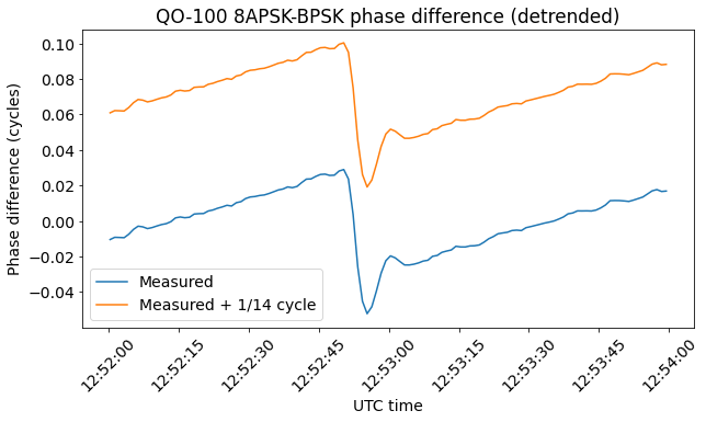
Nevertheless, I am still seeing phase jumps in the measurements. I have thought that occasionally the Costas loop for the BPSK beacon might unlock due other signals interfering with the beacon signal (sometimes people transmit on top of the beacon). When this happens, this Costas loop might lock again in the opposite phase. Then the 8APSK Costas loop will need to lock to a different constellation point (recall that the 8APSK Costas loop is steered by the BPSK Costas loop). The phase difference will jump by a multiple of 1/14 cycle (typically by +/- 1/14 cycle, since the 8APSK Costas loop bandwidth is much lower than the BPSK Costas loop bandwidth, so the 8APSK Costas loop will not move much during the time when the BPSK Costas loop is unlocked).
Most of the phase jumps I am seeing after all the above problems have been solved look like the next figure. The jump is somewhat smaller than 1/14 cycle, so it cannot be explained by this reasoning.
There are some other jumps that seem to be exactly of 1/14 cycle, as shown below.
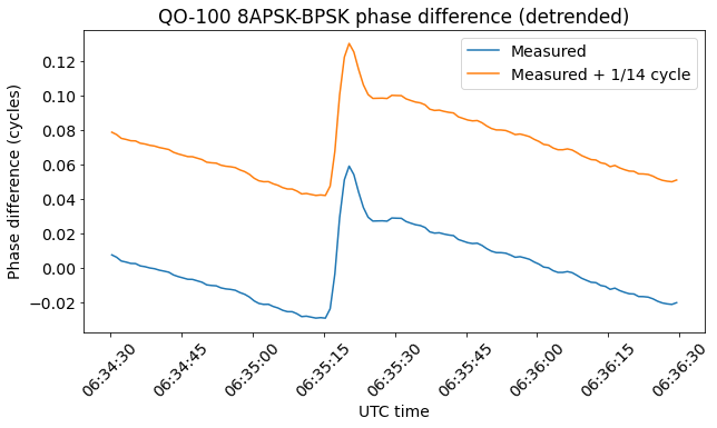
So perhaps there are two different causes for the jumps. One is as described above, and only causes the phase difference to change by a multiple of 1/14 cycle (the phase difference measurement is ambiguous modulo 1/14 cycle, really). The other seems to involve a real change in the group delay being measured, either because samples have been lost in the transmitter or receiver, or because of a true change in the group delay through the transponder (which would be strange but still possible).
It would be interesting if other stations can set this kind of measurement up, since it would indicate if the cause is in my groundstation or somewhere else. In any case, I am not too worried about these jumps, because they happen infrequently (about twice per day) and as we’ll see, they don’t really affect the orbit determination that I’m doing.
I have made a modification to the way that phase measurements are written to a file. Previously, I was writing wrapped phase measurements at 200 sps and doing the unwrap in Python. The reason for using 200 sps is to avoid aliasing with the BPSK beacon phase, since its frequency changes by about 60 Hz due to Doppler. The problem is that the 200 sps files with several days of data were quite large.
Now I have implemented a Phase Unwrap block in C++ and added it to gr-satellites. This block does phase unwrapping by keeping the count of integer cycles in an int64_t variable. The output of the block is the value of the int64_t number of integer cycles and the float fractional phase in radians. By using an int64_t there is no chance for overflows. The block runs at the same rate as the Costas loops (6 ksps), so aliasing is impossible. The output of the block can then be downsampled to any desired rate. I am writing to file the unwrapped phase measurements at a 1 Hz rate. This has the advantage that the output files are much smaller, and loading all the data in Python requires much less RAM.
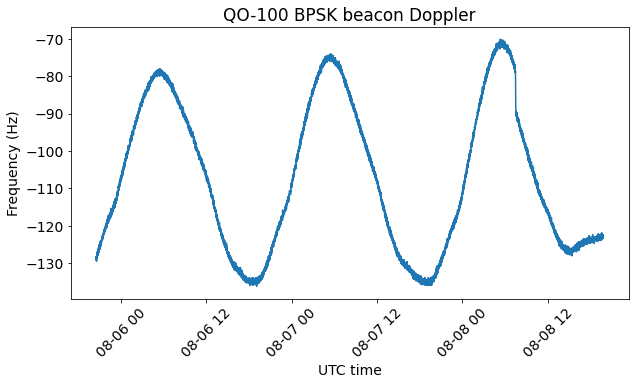
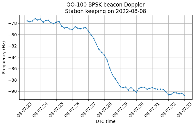
I have been running the new GNU Radio flowgraph for almost 3 days. The Doppler of the BPSK beacon is shown here, we see the daily Doppler sinusoid, which is somewhat distorted by the drift of the local oscillator of the transponder. The sudden jump in Doppler on the morning of 2022-08-08 corresponds to a station keeping manoeuvre.
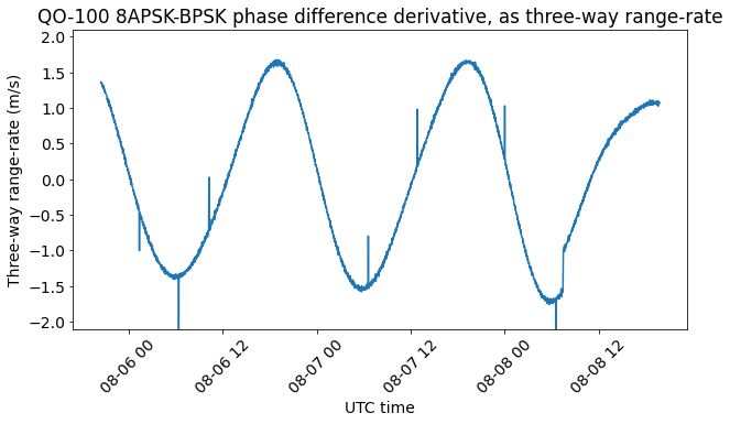
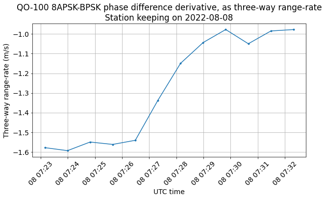
The three-way range-rate, computed as the derivative of the phase difference between the 8APSK and BPSK beacons shows the daily sinusoid curve and no effects from the transponder local oscillator. The glitches correspond to jumps in the phase difference measurements. The integration time used here is 100 seconds.
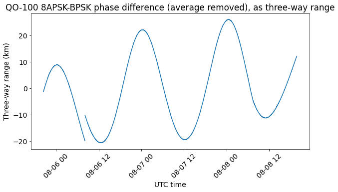
Finally, the plot below shows the three-way range, computed from the phase difference. The average of the measurements has been removed, since there is an unknown constant offset in the measurements. There are two separate traces because the receiver was restarted, and the average has been removed separately for each run (the two runs have different constant offsets). There are small jumps due to the phase jumps, but they are not visible with this scale.
On 2022-08-08 at 07:27 UTC there has been a station keeping manoeuvre. The details of the manoeuvre are shown below in the Doppler and the range-rate. We see that the burn lasted 2 minutes and the range-rate changed by around 0.6 m/s. This corresponds approximately to a projection of 0.3 m/s on the orbit binormal vector, since the line-of-sight vectors from grounstations on Earth are almost aligned with the orbit binormal.
Orbit determination with GMAT
Performing orbit determination with only the three-way range and range-rate data for the transmitting groundstation in Bochum and my receiving groundstation in Madrid is a rather ill conditioned problem. Moreover, our range data has an unknown constant offset, as explained in the previous post. Therefore, I have spent some time messing around with GMAT’s orbit determination to find an approach that works.
The main idea is to start with a TLE from Celestrak as a-priori state for the satellite. However, TLEs are known to describe the Doppler of GEO satellites quite poorly (see this post, for instance). We can already see this by looking at the residuals from the first LSQ iteration of orbit determination or by comparing our data with simulated data in GMAT. The main problem is that the residual vector of the first LSQ iteration throws the state to a completely unfeasible orbit, and then the estimation doesn’t converge.
Even if we try to tweak the Keplerian parameters of the TLE by hand to try to match our data more closely (which is a tedious and tricky task), we still run into problems with the LSQ estimator. I tried to use both the range-rate and range measurements, by determining an appropriate constant offset for the range measurements by hand, and still the estimator failed to converge.
Geometrically, we can see why the problem is so ill conditioned. If we ignore the light-time delay, the three-way range measures the sum of distances between the satellite and Madrid, and the satellite and Bochum. Therefore, for each of the ellipsoids with foci at Madrid and Bochum, we get the same range measurement regardless of which position on that particular ellipsoid the satellite is. Without getting into technical details about fibre bundles and such, this means that we only can measure data along a 1-dimensional manifold, which is orthogonal to the collection of all the ellipsoids with foci at Madrid and Bochum. From this 1-dimensional manifold we are trying to derive the Keplerian parameters for the satellite, which have more degrees of freedom (think of how the sub-satellite point moves in latitude and longitude, tracing some kind of figure 8 curve or a non-periodic curve).
Another way of thinking about this is that if the satellite goes up in altitude (due to a nonzero eccentricity), then the range grows. If the satellite goes south in latitude (due to a nonzero inclination), then the range also grows, because both groundstations are in the northern hemisphere. Therefore, from these measurements it is hard to tell apart the eccentricity vector from the orbit normal vector.
The idea I had to avoid the problems with the LSQ estimation is to try to constrain the state vector by imposing the condition that the position of the satellite must remain close to what indicated by the TLEs. After all, it’s a GEO, so its position in ECEF coordinates won’t change much. To do this, I generate GPS_PosVec observations with GMAT’s simulator. These are the ECEF position vectors that would normally be generated by a GPS receiver on board the spacecraft (see this post about orbit determination with the on-board GPS receiver in the Lucky-7 cubesat). However, in this case we can use them to get artificial constraints for the position of the satellite. These constraints help the LSQ discard absurd solutions, so that it can converge to a reasonable solution for a GEO orbit.
To avoid biasing the solution by the “fake” GPS_PosVec observations, these are generated with a standard deviation of 100 km. The same standard deviation is then used in the the LSQ for these measurements. Therefore, non-GEO orbits that take the satellite out of its GEO position will have a huge least-squares cost and will not be considered by the LSQ. Among the feasible GEO-like orbits, the real observations from the phase difference measurements are used to choose the most likely state vector.
In the end I have used only the range-rate observables. With these plus the GPS_PosVec the LSQ already converges to an LSQ solution that fits more or less well the range-rate. The glitches in the range-rate caused by phase jumps are easily discarded by the OLSE filter.
In the future I might study how to incorporate the range observables. This is more tricky, given that there is a “floating ambiguity” (a constant offset) to be determined, and also the phase jumps. The standard deviation for the range-rate observables is set to 1 cm/s, as this more or less matches what we get with our measurements over 100 second integrations. To get the data into GMAT, I am writing GMD files from the Jupyter notebook where I process the measurements.
In GMAT I am using a force model that considers an 80×80 EGM96 model for the gravity of Earth, the point-mass gravities of the Sun, Moon, Venus, Mars and Jupiter, solar radiation pressure, and relativistic effects. For the solar radiation pressure I am using a spherical model with an area of 16 m², a reflection coefficient of 1.8, and a satellite mass of 5000 kg. These are only very crude estimates.
I have performed LSQ estimation using the range-rate data from 2022-08-05 20:28 UTC to 2022-08-08 07:25, which is just before the station keeping burn. The estimation is done for the Cartesian state of the satellite, because the Keplerian state of a GEO orbit works quite pathologically due to the low inclination and eccentricity. The state vector is defined and printed out in Keplerian state, as it is easier to interpret. The epoch 2022-08-07 00:00:00 UTC is used as the epoch of estimation, as it is more or less in the middle of the estimation arc. The reference frame is MJ2000Eq.
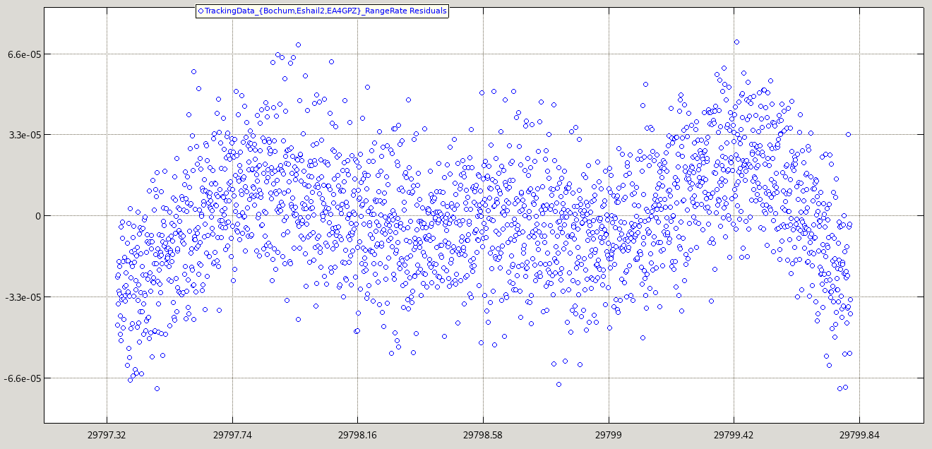
The figure below shows the range-rate residuals after the convergence of the LSQ estimator. The horizontal axis is time in GMAT’s MJD, and the vertical axis is residual in km/s. We can see that the noise is around 1 cm/s, as we indicated, but there is also an unmodeled effect of a few cm/s. It looks like an inverted “W” shape. It will be interesting to study if this effect appears when estimating over other, perhaps longer, time arcs.
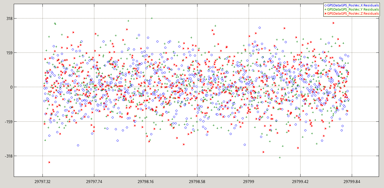
The residuals for the “fake” GPS data do not show any obvious bias due to their large noise (the vertical axis is in km). Note that these were generated with the a-priori state vector from the TLE, so there is indeed a bias hidden in the noise because as we will see below the LSQ solution is somewhat different.
Epoch = 2022-08-07 00:00:00.000 UTC
SMA = 42162.56138119999
ECC = 0.0004584083251553041
INC = 0.04439641847167956
RAAN = 140.236781219
AOP = 29.40313884451632
TA = 171.6576522989836
Compare these with the TLE form Celestrak, which is (in OMM format):
CSDS_OMM_VERS = 2.0
CREATION_DATE  =
ORIGINATOR     =

OBJECT_NAME    = ES'HAIL 2
OBJECT_ID      = 2018-090A
CENTER_NAME    = EARTH
REF_FRAME      = TEME
TIME_SYSTEM    = UTC
MEAN_ELEMENT_THEORY = SGP/SGP4

EPOCH          = 2022-08-05T18:32:42.732384
MEAN_MOTION    = 1.00271717
ECCENTRICITY   = .0001738
INCLINATION    = 0.0129
RA_OF_ASC_NODE = 91.9843
ARG_OF_PERICENTER = 78.3235
MEAN_ANOMALY   = 87.9470

EPHEMERIS_TYPE = 0
CLASSIFICATION_TYPE = U
NORAD_CAT_ID   = 43700
ELEMENT_SET_NO = 999
REV_AT_EPOCH   = 1352
BSTAR          = 0
MEAN_MOTION_DOT = .15E-5
MEAN_MOTION_DDOT = 0
I have transformed this into a GMAT Keplerian state by ignoring the difference between TEME and MJ2000Eq and making the true anomaly equal to the mean anomaly, since the orbit is almost circular. This gives
SMA = 42164.79643866292
ECC = 0.0001738
INC = 0.0129
RAAN = 91.9843
AOP = 78.3235
TA = 87.9470
The difference in true anomaly between the TLE and the estimated estate is to be expected, since the two states use different epochs. However note that the estimated eccentricity is 2.6 times larger than the one in the TLE, and the inclination of the estimated state is 4.4 times larger. The RAAN has also changed significantly. On the other hand, the right-ascension of the perigee (which is the thing we should look at for comparison, rather than argument of perigee) hasn’t changed that much (169.6 deg versus 170.3 deg, assuming zero inclination and eccentricity for this calculation).
The correlation matrix of the estimated state in Keplerian coordinates is
 1.00  0.01  0.01  0.02 -0.02  0.02
 0.01  1.00 -0.40  0.91 -0.83  0.00
 0.01 -0.40  1.00  0.00 -0.17  0.91
 0.02  0.91  0.00  1.00 -0.99  0.41
-0.02 -0.83 -0.17 -0.99  1.00 -0.55
 0.02  0.00  0.91  0.41 -0.55  1.00
The order of the coordinates is SMA, ECC, INC, RAAN, AOP, and MA. We see that there are really high correlations between ECC and RAAN and AOP. Likewise, in the Cartesian state there is a high correlation between X, Y and VX, and also between Y, VX and VY (but not between X and VY).
Code and data
The GNU Radio flowgraph is qo100_beacon_phase.grc. The measurements are processed in this Jupyter notebook. The measurement files are included in the repository. The GMAT script is qo100_orbit_determination.script. It has been run with the data in this GMD file.
One comment