In a previous post, I showed my orbit determination experiments of the GEO satellite Es’hail 2 using the beacons transmitted from Bochum (Germany) through the QO-100 amateur radio transponder on-board this satellite. By measuring the phase difference of the BPSK and 8APSK beacons, which are spaced apart by 245 kHz in the transponder, we can compute the three-way range-rate between the transmitter at Bochum and my receiver in Spain. This data can then be used for orbit determination with GMAT.
I have continued collection more data for these experiments, so this post is an update on the results.
First I should point out an error in the previous post. I had left an extra 20 uHz term in the frequency separation correction, which I used during my tests about measuring the frequency separation exactly. However, this term doesn’t seem to affect the orbit-determination with range-rate by that much. The error corresponds to some 24 mm/s of error in the range-rate, which is comparable to the residual standard deviation that we get. I have now run again the orbit determination with the correct data.
Another change with respect to the previous post is that now I am using the TODEq (true of date equatorial) reference system rather than the MJ2000Eq (mean J2000 epoch equatorial) system for the spacecraft state vector. The difference between the two is described in Section 2.5 of GMAT’s mathematical specification. Compared to MJ2000Eq, TODEq includes precession and nutation. For this reason, TODEq is the ECI (Earth centred inertial) system whose z-axis is closest to that of the ITRF ECEF (Earth centred Earth fixed) system (note that because TODEq includes precession and nutation, strictly speaking it is not an inertial system). The transformation between TODEq and ITRF involves only the rotation about the z-axis corresponding to sidereal time, and polar motion (which is a small rotation that changes the z-axis).
Using the TODEq system gives an easier interpretation of the GEO orbit. A perfect GEO orbit will have fixed coordinates in ITRF. In particular the satellite will be on the ITRF equator. The ITRF equator is very close to the TODEq equator, so the inclination of the orbit in TODEq coordinates should be very small. In contrast, the TODEq equator and the MJ2000Eq equator differ by a fraction of a degree, so the inclination of such a perfect GEO orbit in MJ2000Eq coordinates would be a fraction of a degree.
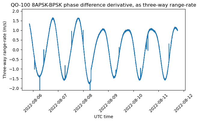
By now I have two sets of measurements. The first is the one that I treated in the previous post, but continues until 2022-08-12, when I stopped the measurements and went on holidays. The range-rate can be seen below. Note that there was a station-keeping manoeuvre on 2022-08-08.
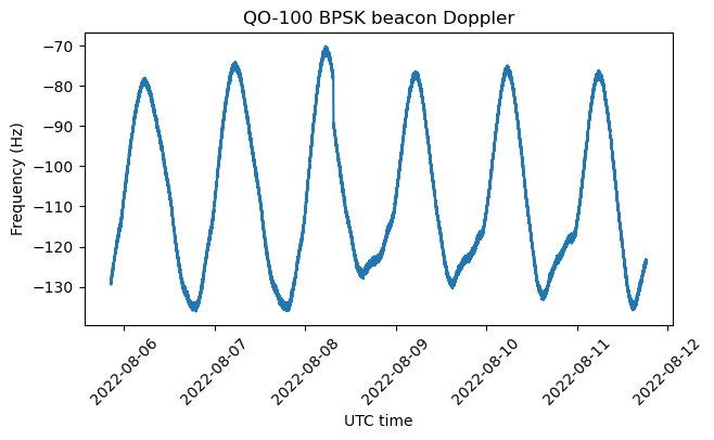
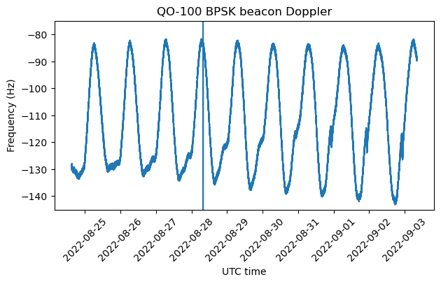
For comparison, here is the Doppler measured on the BPSK beacon. This is affected by the drift of the transponder local oscillator, so it is not very useful for orbit determination.
To perform orbit determination, I am dividing the data in two arcs: before and after the manoeuvre. I am using some Python code to read the report files generated by GMAT and plot the residuals. This gives me more control over the plots than what is plotted in the GMAT GUI (see the previous post).
The figure below shows the plot corresponding to the arc before the manoeuvre. The first plot shows the range-rate residuals in mm/s. The measurements that have been used for the least-squares fit are shown in blue, while the measurements that have been discarded, either by data selection or by the OLSE filter, are shown in orange. The bottom plot shows some data computed from the ECEF coordinates of the satellite in the orbit determination solution: the difference between the orbit radius and the nominal radius of 42164 km for a GEO orbit is shown in blue, the ECEF z-coordinate is shown in orange, and the longitude is shown in green. These indicate how the orbit deviates from a perfect GEO orbit because of a non-zero eccentricity and inclination.
The sinusoids affecting the longitude and the orbit radius should always be in quadrature because of Kepler’s third law. The phase difference between the sinusoids of the orbit radius and the ECEF z-coordinate depends on the argument of perigee. The phase of the z-coordinate sinusoid with respect to time depends on the right-ascension of the ascending node and the time of the year.
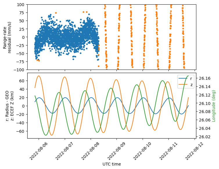
As in the previous post, we observe that the residuals have a small M-shaped bias. In fact, we will find this kind of oscillation in the residuals of all the estimation arcs. This hints at some effect which is not taken into account by the GMAT model.
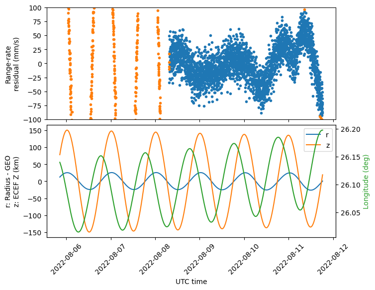
The results for the arc following the station-keeping burn are shown next. Note the wavy pattern in the residuals. In the ECEF coordinates we can see that the main change is in the amplitude of the z-coordinate oscillation. This means that the inclination has increased.
Below we show the Keplerian state for the estimation solutions of the arc before the manoeuvre and after the manoeuvre (the estimation is done for Cartesian state, but the Keplerian state is easier to interpret). For each parameter, both its value and standard deviation are shown. The RAAN and AOP have relatively large standard deviations of a few degrees, because as we mentioned in the the previous post the geometry of a single three-way measurement baseline is not so good to tell apart the eccentricity vector from the orbit normal vector.
The main change that we observe due to the manoeuvre is that the inclination has increased greatly (it has doubled). The eccentricity has also increased somewhat.
Estimation Epoch : 07 Aug 2022 00:00:00.000 UTCG
SMA  km  42164.87700873 2.10216603e-02
ECC      0.00044664     1.31431672e-05
INC  deg 0.09592203     6.35351048e-03
RAAN deg 250.66401205   7.63560226e+00
AOP  deg 278.97431565   8.60138151e+00
MA   deg 171.93512335   1.69246492e+00

Estimation Epoch : 10 Aug 2022 00:00:00.000 UTCG
SMA  km  42164.87332818 1.75285852e-02
ECC      0.00057374     8.63979604e-06
INC  deg 0.18618296     4.17385673e-03
RAAN deg 255.63979613   3.26306773e+00
AOP  deg 278.95740291   2.54711522e+00
MA   deg 169.96528258   8.66346445e-01
The next set of measurements starts on 2022-08-24, when I returned from holidays. The measurements continue until 2022-09-02 20:35 UTC, when the 8APSK beacon went offline. The beacon continues to be off as of writing this post. I have divided this set into several arcs of 4 days. Trying to use longer arcs gives problems because of the unmodelled effect that gives a wavy pattern in the residuals. In fact, in this set of measurements we can see this effect better, because we can see the wavy pattern in the residuals growing as we go away from the arc that was used for estimation.
The figure below shows the Doppler of the BPSK beacon. Note that, unlike the 8APSK beacon, the BPSK beacon has continued running even after 2022-09-02 20:35 UTC. There seems to be a short time interval on 2022-08-28 when the BPSK beacon was either off or interfered by another signal.
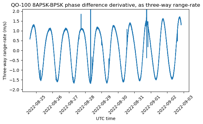
The next figure shows the three-way range-rate computed from the phase difference measurements. As usual, there are some glitches that will be filtered by the OLSE.
The next figures show the results of the estimation for the three 4-day arcs the we’re considering: 2022-08-25 – 2022-08-29, 2022-08-28 – 2022-09-01, and 2022-08-31 – 2022-09-03. Note how the oscillation of the residuals keeps growing as we get farther from the estimation interval. Additionally, the phase of the oscillation reverses as we cross over the estimation interval. Note that the oscillation is roughly in phase with the ECEF z-coordinate after the estimation interval, and in anti-phase before the estimation interval.
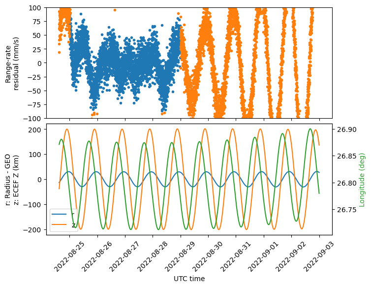
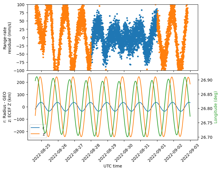
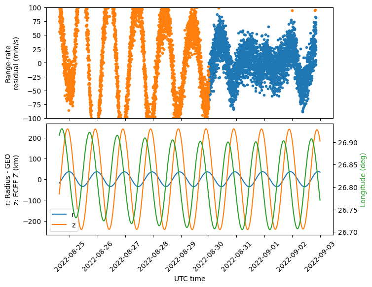
The Keplerian state for each of the estimation arcs is shown below. Comparing these, it seems that there is an increase over time in both eccentricity and inclination. I think this is related to the unmodelled effect that causes a wavy pattern in the residuals.
Estimation Epoch : 27 Aug 2022 00:00:00.000 UTCG
SMA  km  42166.60094819 1.57418011e-02
ECC      0.00063954     6.02263472e-06
INC  deg 0.26976590     2.98192608e-03
RAAN deg 233.85323270   9.38115060e-01
AOP  deg 292.00626619   6.01234428e-01
MA   deg 196.14439872   5.76399754e-01

Estimation Epoch : 30 Aug 2022 00:00:00.000 UTCG
SMA  km  42166.82492251 1.57486474e-02
ECC      0.00077555     5.43147020e-06
INC  deg 0.33264776     2.69422534e-03
RAAN deg 239.01234432   6.50651842e-01
AOP  deg 286.50501933   3.33149090e-01
MA   deg 199.44769691   4.19306563e-01

Estimation Epoch : 01 Sep 2022 00:00:00.000 UTCG
SMA  km  42166.46033380 1.60350557e-02
ECC      0.00080055     5.73869011e-06
INC  deg 0.32800769     2.81267044e-03
RAAN deg 239.16142829   6.93951667e-01
AOP  deg 285.05091539   3.63936867e-01
MA   deg 202.73043611   4.19816545e-01
It is not so easy to think geometrically about the oscillation that appears in the residuals, because the three-way range-rate is the combination of several oscillatory terms. For instance, the time derivative of the orbit radius gives a positive contribution to the range-rate, but the time derivative of the ECEF z-coordinate gives a negative contribution, because both Madrid and Bochum are in the northern hemisphere. Since the oscillations of these two terms are roughly in phase, they cancel out to some extent. The range-rate is more or less in phase with the derivative of the orbit radius. This means that the effect of the orbit radius dominates that of the z-coordinate.
Since Madrid and Bochum are west of the satellite, the time derivative of the longitude oscillations also gives a positive contribution to the range-rate. We notice that the range-rate residuals oscillation has roughly the same phase as the time derivative of the longitude before the estimation interval, and opposite phase after the estimation interval. This hints to a decrease in the amplitude of the longitude oscillations over time. However, this doesn’t match with the orbit determination results, because the longitude oscillations are proportional to the eccentricity, which seems to be increasing over time.
Arguably, the phase of the range-rate residuals is also close to the phase of the range-rate itself (opposite phase before the estimation arc, and the same phase after the estimation arc). This might suggest that the quantity that is growing in amplitude is the range-rate, rather than the longitude oscillations being decreasing in amplitude. This idea makes more sense in view of the growth in eccentricity and inclination.
The data and code used in this post can be found in the usual repository.