GUPPI stands for Green Bank Ultimate Pulsar Processing Instrument. The GUPPI raw file format, which was originally used by this instrument for pulsar observations, is now used in many telescopes for radio astronomy and SETI. For instance Breakthrough Listen uses the GUPPI format as part of the processing pipeline, as described in this paper. The Breakthrough Listen blimpy tools work with GUPPI files or with filterbank files (basically, waterfalls) that have been produced from a GUPPI file using rawspec.
I think that GNU Radio can be a very useful tool for SETI and radio astronomy, as evidenced by the partnership of GNU Radio and SETI Institute. However, the set of tools used in the GNU Radio ecosystem (and by the wider SDR community) and the tools used traditionally by the SETI community are quite different, and even the file formats and some key concepts are unalike. Therefore, interfacing these tools is not trivial.
During this summer I have been teaching some GNU Radio lessons to the BSRC REU students. As part of these sessions, I made gr-guppi, a GNU Radio out-of-tree module that can write GUPPI files. I thought this could be potentially useful to the students, and it might be a first step in increasing the compatibility between GNU Radio and the SETI tools. (The materials for the sessions of this year are in this repository, and the materials for 2021 are here; these may be useful to someone even without the context of the workshop-like sessions for which they were created).
In this post I will show how gr-guppi works and what are the key concepts for GUPPI files, as these files store the output of a polyphase filterbank, which many people from the GNU Radio community might not be very familiar with. The goal of the post is to generate a simulated technosignature in GNU Radio (a CW carrier drifting in frequency) and then detect it using turboSETI, which is a tool for detecting narrowband signals with a Doppler drift.
Before going on, it is convenient to mention that an alternative to this approach is using gr-turboseti, which wraps up turboSETI as a GNU Radio block. This was Yiwei Chai‘s REU project at the ATA in 2021.
Polyphase filterbanks
GUPPI files store IQ data, or as astronomers call it, voltage-mode data (in contrast to waterfall-like data, which has already been power detected). However, they are fundamentally different from the raw IQ files used by much of the SDR community (i.e., files handled by the File Sink and File Source GNU Radio blocks, SigMF files, IQ WAV files, etc.) This is because GUPPI files store the output from a polyphase filterbank, whereas the other file types consist of a single channel of IQ data.
Therefore, it is convenient to have some notion of how polyphase filterbanks work, and why they are so useful in radio astronomy. Polyphase filterbanks form part of the signal processing pipeline of most telescopes. They are performed as one of the first steps after signal digitization, usually in an FPGA. Often, raw ADC data is not accessible to the telescope user, so GUPPI raw file, or another file storing the output of the polyphase filterbank is the rawest kind of data that can be obtained from the telescope.
A polyphase filterbank is a way of channelising an IQ signal at sample rate \(f_s\) into \(N\) channels each having sample rate \(f_s/N\). These channels are equally spaced and cover the whole Nyquist bandwidth \((-f_s/2, f_s/2)\), so the channel spacing is \(f_s/N\). We can think of the effect of the polyphase filterbank for each of these channels as applying a bandpass filter to the original signal, shifting down to baseband, and decimating by a factor of \(N\).
For simplicity, here we only treat critically sampled polyphase filterbanks (i.e., those in which the channel spacing and output sample rate of each channel are equal) applied to IQ (complex) signals. With suitable modifications, it is possible to consider also real signals, and non-critically sampled polyphase filterbanks, in which the output sample rate of each channel is larger than the channel spacing.
For each \(N\) samples that go in, the polyphase filterbank outputs one sample for each of the \(N\) output channels, so the total amount of samples is conserved. A good way to think about the output of the polyphase filterbank is that it is time-frequency domain data. The \(N\) channels correspond to different frequencies, but if we look at the consecutive samples of the same channel, those give time-domain IQ data in the usual sense for that particular channel. Some example applications of the polyphase filterbank output help illustrate this:
- If our signal of interest is entirely contained in one of the channels, we can use only the output samples for that channel as regular time-domain IQ data and ignore the remaining channels.
- If we compute the average power of each of the channels separately (by computing the average of the modulus squared of the samples), then we obtain the power spectrum, with each of the channels representing a different frequency bin.
In this sense, polyphase filterbanks may seem quite similar to an FFT, in the sense that an \(N\)-point FFT can be used to perform this operation of channelization into \(N\) channels in time-frequency domain. Polyphase filterbanks are in fact some kind of “glorified” FFT, in the sense that they consist of an \(N\)-point FFT plus some FIR filter stuff before the FFT. The disadvantage of using an FFT for channelization is the spectral leakage and scalloping loss. These cause the frequency response of the filter applied to each channel to be far from ideal. A suitable window function can be used to improve this, but polyphase filterbanks give even better control that is not possible with a windowed FFT.
The figure below, taken from fred harris‘ book Multi-rate Signal Processing for Communication Systems, shows some of the different channel filter shapes that can be obtained with a polyphase filterbank depending on the intended application. The reader interested in all the mathematical details of polyphase filterbanks, with an emphasis on practical applications, can consult Chapter 9 in this book.
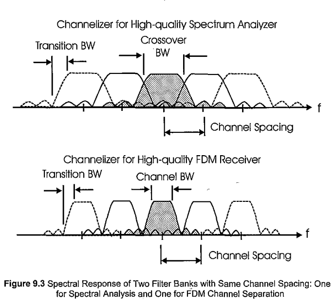
The channel filter is designed as a regular lowpass FIR filter with \(Nk\) taps. This filter is called prototype filter, since it is then used to generate each of the channel filters by shifting it in frequency. The factor \(k\) determines the number of multiplications required per input sample. In radio astronomy it is typical to use a small value such as \(k = 4\) or \(k = 8\). Larger values of \(k\) will give a filter with better characteristics, but will require more FPGA resources. The lowpass filter should have a cut-off frequency somewhat below \(f_s/(2N)\), since the output Nyquist frequency will be \(f_s/(2N)\). Everything which is further away than \(f_s/(2N)\) from the centre frequency of each channel and is not stopped by this filter will produce aliasing. Ideally we would like to have a brick-wall filter with a cut-off of \(f_s/(2N)\), but since this is impossible, we need to balance factors such as the how close we make the cut-off frequency to \(f_s/(2N)\), how large is the transition bandwidth, and how much stop-band attenuation we get. The best trade-off will depend on the intended application.
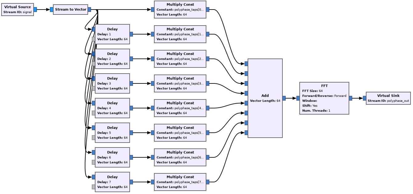
The figure below shows a way of implementing a polyphase filterbank in GNU Radio. This is taken from the guppi_sink_example.grc example in gr-guppi. We see that first there is some slightly funny FIR filter thing using a variable polyphase_taps (refer to the book by fred harris for details). This part has 8 branches because we are using \(k = 8\). Then there is an 64-point FFT block, since we are using \(N = 64\) channels.
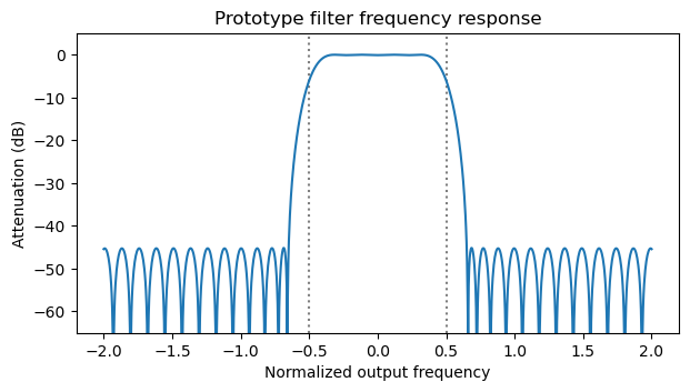
The prototype filter, polyphase_taps is designed using the Remez algorithm from scipy as
scipy.signal.remez(
    num_taps,
    [0, 0.35/num_channels, 0.65/num_channels, 0.5],
    [1, 0])
Here num_taps corresponds to the product \(Nk = 512\), and num_channels is \(N = 64\). The frequency response of this filter can be seen below.
Polyphase filterbanks in radio astronomy
Polyphase filterbanks are very useful and common in radio astronomy. There are a number of reasons for this, which help understand how they are used.
First, radio telescopes usually handle very large bandwidths. Dividing the signal into frequency channels is a good way to perform work in parallel, for example, by assigning different sets of channels to different machines for storage to disk or further real-time processing. This frequency-domain division is helpful because many processing tasks can be done independently for each of the frequency channels. On the contrary, a time-domain division is not so helpful for parallelizing tasks.
For example, the current backend of the Allen Telescope Array, which is based on RFSoC boards, performs real sampling at 2048 Msps. A 4096 channel polyphase filter bank is used to obtain 0.5 MHz wide channels. Of these, only 2049 channels are necessary due to the spectral symmetry of a real signal. Moreover, not all the 1024 MHz bandwidth is of interest, because the telescope IF is approximately 700 MHz wide and centred at 512 MHz. Each set of 192 consecutive channels (96 MHz of bandwidth) is processed by a different machine. Take into account that currently the ATA backend uses 20 antennas (each with two polarizations) and two IF tunings. This will be scaled up to 42 antennas and four IF tunings in the future. For each set of 192 channels, the data for all of the antennas and one IF tuning is sent to the same machine, since the beamformer and correlator need access to all of the antennas. Different IF tunings are handled in different machines.
Another reason has to do with calibration. Many calibrations depend on frequency. For instance, an amplitude and phase calibration applies a frequency-dependent correction. If the output channels from the polyphase filterbank are narrow enough (between a fraction of a MHz and a few MHz), the calibration can be applied as a frequency-independent value in each frequency channel. This also serves for the delay and phase corrections that are needed for beamforming. Additionally, in pulsar and FRB processing it is common to perform de-dispersion. The electrons in the interstellar medium introduce a frequency-dependent delay in the signal, so that the lower frequencies of the pulse arrive later. By delaying differently each of the polyphase filterbank channels, the effect of dispersion can be corrected and the pulse can be aligned again (there exists also a more complicated coherent de-dispersion algorithm).
An idea related to calibration is that of data reduction by reducing the number of bits. By using few bits (2 or 4) to quantize the amplitude of the signal, the data to handle is reduced. However, if we only use a few bits, we cannot have a large dynamic range for the amplitudes. Here a polyphase filterbank can help. Each of the output channels can be normalized in amplitude before being quantized with few bits. The amplitude normalizations for each channel can use more bits, as they change less frequently. This normalization is usually considered as part of the calibration, as it performs amplitude versus frequency equalization. This technique is perhaps falling a bit out of use, because many telescopes can now afford to use 8 bit quantization. It was used with the older SNAP boards in the ATA (see Section 2.5.5 in the SNAP user manual).
A polyphase filterbank is useful for spectrometry. In this observing mode, only the power spectral density of the signal is calculated and recorded. If only coarse frequency resolution is needed, the average power of each of the output channels can be computed. For a finer resolution, an FFT can be used with the output of each channel. This approach of channelizing the signal in two steps, first with a polyphase filterbank and then with an FFT, avoids the very large FFT sizes that would be needed to obtain a fine frequency resolution (say 1 Hz) with a signal of large bandwidth (say 1 GHz). We will show an example of this application below, when we use rawspec to compute waterfall data.
Finally, another reason is that a polyphase filterbank can be used as the “F part” of an FX correlator. In this correlator architecture, the complex voltage data from each antenna is first passed to time-frequency domain with a polyphase filterbank or FFT, and then the products \(x_j(f)\overline{x_k(f)}\) are calculated and averaged in time for each pair of antennas \((j,k)\). This approach is perhaps the most popular today because it has some advantages with respect to the XF approach, in which the signals are first multiplied in the time domain, and then the products are passed to time-frequency domain. In particular, the FX correlator scales better with the number of antennas.
GUPPI files
A GUPPI file is a binary file that contains the output from a polyphase filterbank. This page gives some notes describing the format. A GUPPI file can store one or two polarizations, but it is a single-antenna format.
The file is organized by blocks. Each block starts with a header that contains several lines of ASCII text, each listing a variable name and a value. These give the format and metadata of the file (number of channels, number of bits, sampling rate, observing frequency, source name and sky coordinates, telescope name, etc.). There are many variables that can be used for metadata. Appendix B in this paper describes the ones that are used in Breakthrough Listen.
After the header, there is a block of binary data containing several samples from each of the output channels of the polyphase filterbank. They are stored as an array ordered by channel, time, and polarization.
The block size of the GUPPI file determines how many samples from each channel are stored in each block. As we will see below, this can be an important parameter. For example, rawspec, which is used to compute a waterfall from a GUPPI file, requires that the product of the FFT size and the number of integrations to perform divides evenly the number of samples per channel in each block.
GUPPI File Sink block
For the time being, the only block that gr-guppi contains is a GUPPI File Sink block. This block can be used to write GUPPI files, similarly to how the File Sink is used to write raw IQ files. The input of the GUPPI File Sink is of vector type, since it should be the output of a polyphase filterbank. Only 8 bit quantization is supported, so the input samples are given already as Char type.
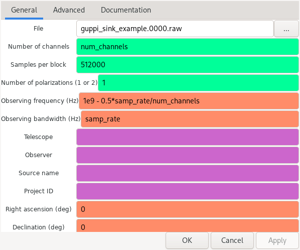
The GUPPI File Sink block is shown below. The number of channels parameter gives the number of polyphase filterbank channels and determines the size of the input vectors. The samples per block is the number of samples of each channel in each of the blocks of the GUPPI file.
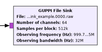
The observing frequency is slightly tricky to get correctly, since it does not refer to the centre frequency of the centre channel. It is actually the leftmost frequency of the centre channel. Therefore, it should be the centre frequency minus 1/2 of the channel width. In this example, the centre frequency is 1 GHz, and the channels are 0.5 MHz wide, so we specify the observing frequency as 999.75 MHz.
In the parameters of the block we can set some metadata regarding the observed source and the telescope. If needed, more metadata fields could be added.
The name of the output file can be chosen freely, but for compatibility with rawspec, contiguous files in the same observation should end with .0000.raw, .0001.raw, etc. Since the GUPPI File Sink writes all the data to a single file, it is best to end the filename with .0000.raw.
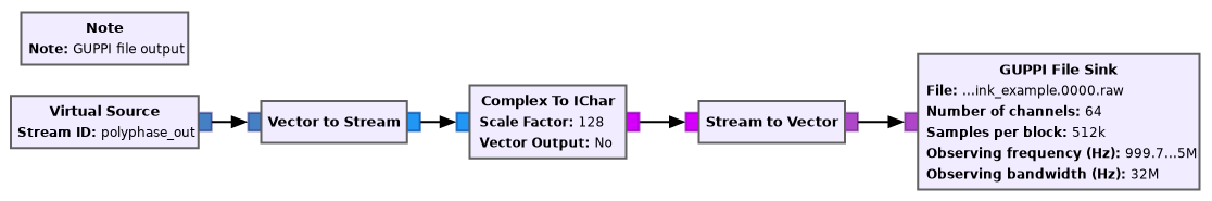
As mentioned above, the input data type for the GUPPI File Sink is a vector of Char samples. Usually, we will be working with Complex samples. The flowgraph below shows how to perform the conversion from the output of the polyphase filterbank. Since Complex To IChar doesn’t work with vectors, we need to use Vector to Stream and Stream to Vector. The Vector to Stream block uses a vector length equal to the number of channels (64 in this case), while the Stream to Vector uses a length equal to twice the number of channels (128 in this case), since the I and Q are stored in two Char samples.
gr-guppi example
The guppi_sink_example.grc flowgraph in gr-guppi shows how to use the GUPPI File Sink block. We have already shown the sections of this flowgraph corresponding to the polyphase filterbank, the conversion to Char, and the GUPPI File Sink.
The input signal for the polyphase filterbank is generated as shown below. It is a chirp in AWGN. The chirp takes 10 seconds to go through the 3 channels in the middle of the filterbank. This kind of signal is quite useful to test that the filterbank and GUPPI file format are implemented correctly. The flowgraph uses a sample rate of 32 Msps and 64 channels, giving a bandwidth of 0.5 MHz per channel.
If we run this example for about 10 to 20 seconds, we will produce a GUPPI file with the chirp signal.
rawspec and watutil
The GUPPI file can be converted to a filterbank file using rawspec. This filterbank file contains waterfall data. The rawspec tool will use the GPU perform an FFT on each channel and sum the modulus squared of several consecutive FFTs. The output can be saved in SIGPROC format, which typically uses the extension .fil, or in HDF5 format, which uses the extension .h5.
We can produce a HDF5 filterbank file for the guppi_sink_example.0000.raw GUPPI file generated by the example flowgraph by running
rawspec -j -f 256 -t 25 guppi_sink_example
The -j parameter selects HDF5 format, the -f parameter sets the FFT size (so we use 256 points per channel, obtaining a frequency resolution of 1953.125 Hz), and the -t parameter sets the number of time integrations (how many consecutive FFTs are added together). In this case, we obtain a resolution of 0.0128 s by using 25 integrations. Note that we indicate the filename without the .0000.raw extension, since rawspec will attempt to open and concatenate the data for files with the extensions .0000.raw, .0001.raw, etc. The output HDF5 file is called guppi_sink_example.rawspec.0000.h5.
The filterbank file can be plotted with the tool watutil from blimpy. To generate all the plots, we can run
watutil -p a guppi_sink_example.rawspec.0000.h5
watutil displays a matplotlib window in which the plots can be panned and zoomed around (click on the image below to see in full size). The main plot is the waterfall, which gives power versus frequency and time using colour.
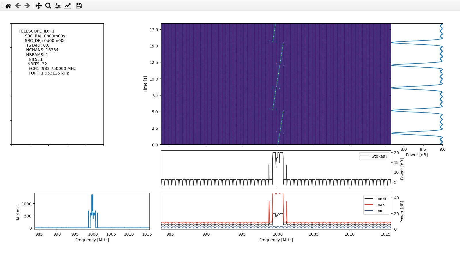
In the waterfall, we can see the edges of the polyphase filterbank channels, and we can also see some aliasing of the chirp in neighbouring channels when it is close to the edge of one channel. Command line parameters can be used to select the types of plots to produce and the region of the data to consider. For instance, we can plot the waterfall of the 7 central channels with
watutil -p w -b 998.25 -e 1001.75 guppi_sink_example.rawspec.0000.h5
(the -b and -e parameters select the frequency range in MHz). This gives the following plot, where we can see more clearly the aliasing effects.

Producing a technosignature signal
Technosignature signals to be detected by turboSETI consist of narrowband signals with a Doppler drift. A chirp that slowly changes its frequency linearly with time is an ideal artificial signal to test turboSETI. Typically, only signals with drifts of up to a few 10’s of Hz/s are considered (see this paper and this paper for estimates of the maximum drift rates that are physically feasible). Additionally, drift rates very close to zero are omitted from the search to avoid detecting carriers at a constant frequency caused by RFI.
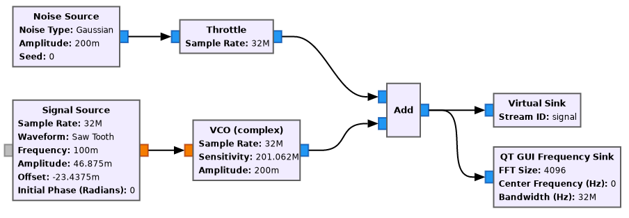
To use turboSETI succesfully, we need to change the parameters of the example to reduce the Doppler drift to something that is reasonable, such as 2 Hz/s. I have set up the parameters of the Signal Source and VCO as shown below.
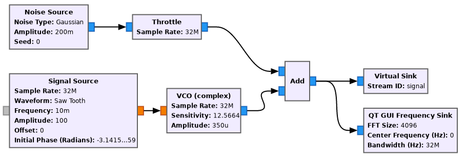
I have reduced the frequency of the Saw Tooth Signal Source to 0.01 (giving a period of 100 seconds) so that we can produce a few tens of seconds of data without having the chirp jumping back in frequency. The amplitude of the saw tooth is 100, so the saw tooth output simply counts time in seconds. I have also set the initial phase to \(-\pi\) to make the saw tooth start at zero (the offset), rather than at the amplitude divided by 2.
For the VCO, we can compute the sensitivity as \(2\pi\) times the drift rate (2 Hz/s), because the sensitivity has units of radians/sec/input value. I have also reduced the amplitude of the VCO to give a weaker signal which is more challenging to detect (around 20 dB·Hz CN0 in this case).
Additionally, I have set the samples per block of the GUPPI file to \(2^{20}\), since we will do with rawspec long FFTs having a length of a power of two. Now the flowgraph can be run for 20 seconds or so to produce a new GUPPI file.
Running turboSETI
turboSETI performs a search of signals with Doppler drift in a filterbank file, so first we must use rawspec to obtain a HDF5 filterbank file from the GUPPI file. We need an adequate time-frequency resolution for the waterfall, according to the type of signal we want to detect. We use an FFT size of \(2^{18}\), which gives a frequency resolution of 1.9 Hz, and 2 integrations, which gives a time resolution of around 1 second. We run rawspec as follows.
rawspec -j -f 262144 -t 2 guppi_sink_example
The next step is to run turboSETI. We can use the -g y parameter to indicate turboSETI to use the GPU, which is much faster. turboSETI gives the following output while it runs. Note that there is a top hit with a drift rate of 1.53 Hz/s, which is close to the drift rate of 2 Hz/s that we used to generate our signal.
$ turboSETI -g y guppi_sink_example.rawspec.0000.h5

turbo_seti version 2.3.2
blimpy version 2.1.3
h5py version 3.7.0
hdf5plugin version 3.3.1
HDF5 library version 1.12.2


data_handler    INFO     From nfpc=262144, n_fine_nchans=16777216 and n_coarse_chan=64
HDF5 header info: {'DIMENSION_LABELS': array(['time', 'feed_id', 'frequency'], dtype=object), 'az_start': 0.0, 'data_type': 1, 'fch1': 983.75, 'foff': 1.9073486328125e-06, 'ibeam': -1, 'machine_id': 20, 'nbeams': 1, 'nbits': 32, 'nchans': 16777216, 'nfpc': 262144, 'nifs': 1, 'rawdatafile': 'guppi_sink_example.0000.raw', 'source_name': '', 'src_dej': <Angle 0. deg>, 'src_raj': <Angle 0. hourangle>, 'telescope_id': -1, 'tsamp': 1.048576, 'tstart': 0.0, 'za_start': 0.0}

Starting ET search with parameters: datafile=guppi_sink_example.rawspec.0000.h5, max_drift=10.0, min_drift=1e-05, snr=25.0, out_dir=./, coarse_chans=, flagging=False, n_coarse_chan=64, kernels=None, gpu_id=0, gpu_backend=True, blank_dc=True, precision=1, append_output=False, log_level_int=20, obs_info={'pulsar': 0, 'pulsar_found': 0, 'pulsar_dm': 0.0, 'pulsar_snr': 0.0, 'pulsar_stats': array([0., 0., 0., 0., 0., 0.]), 'RFI_level': 0.0, 'Mean_SEFD': 0.0, 'psrflux_Sens': 0.0, 'SEFDs_val': [0.0], 'SEFDs_freq': [0.0], 'SEFDs_freq_up': [0.0]}

Computed drift rate resolution: 0.10699937667916803

find_doppler.0  INFO     Spectra 0 1st 3 values: [171.82579041 176.84150696 125.91470337]
find_doppler.0  INFO     Spectra 1 1st 3 values: [140.18817139  96.32918549 209.73249817]
find_doppler.32 INFO     Top hit found! SNR 178.919785, Drift Rate 1.525604, index 131072
Search time:  0.09 min
turboSETI produces the file guppi_sink_example.rawspec.0000.dat, which contains a list of the hits that have been detected. We see that the hit is at a frequency of 1000 MHz, which coincides with the frequency of our technosignature signal.
# -------------------------- o --------------------------
# File ID: guppi_sink_example.rawspec.0000.h5
# -------------------------- o --------------------------
# Source:
# MJD:     0.000000000000	RA: 0h00m00s	DEC: 0d00m00s
# DELTAT:   1.048576	DELTAF(Hz):   1.907349	max_drift_rate:  10.000000	obs_length:  18.874368
# --------------------------
# Top_Hit_# 	Drift_Rate 	SNR 	Uncorrected_Frequency 	Corrected_Frequency 	Index 	freq_start 	freq_end 	SEFD 	SEFD_freq 	Coarse_Channel_Number 	Full_number_of_hits
# --------------------------
000001	  1.525604	178.919785	   1000.000000	   1000.000000	131072	    999.999348	   1000.000650	0.0	      0.000000	32	225
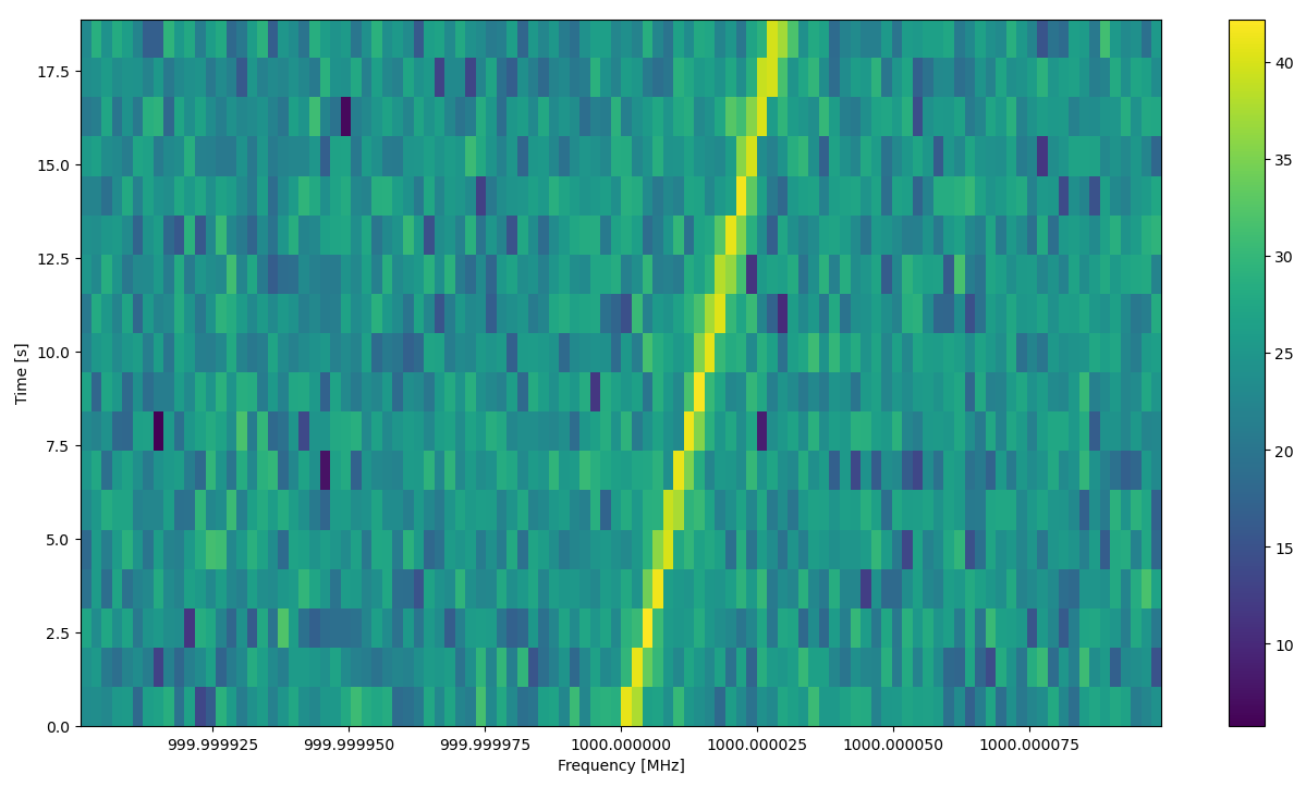
We can run
watutil -p w -b 999.9999 -e 1000.0001 guppi_sink_example.rawspec.0000.h5
to show the waterfall in a 200 Hz span around 1000 MHz. This gives the following plot, where we can see the signal drifting in frequency.
Conclusions
Here we have shown how the GUPPI File Sink block from gr-guppi can be used to produce files that can be processed with the Breakthrough Listen tools rawspec, watutil and turboSETI. I think that GNU Radio is a very valuable addition to the ecosystem of SETI tools.
As shown by the example above, GNU Radio can be a good tool to generate simulated signals to test the tools. For example, it can help test turboSETI to see which SNRs are required to detect signals depending on the time-frequency resolution and the drift rate. A simple chirp can be generated as above. The frequency of this chirp changes linearly with time. Also, the Doppler correction block from gr-satellites could be used to generate a signal with an arbitrary Doppler curve, by reading the data from a file.
The capability to read GUPPI files in GNU Radio would also be interesting, so I might add a GUPPI File Source in the future. This would allow for instance reading the data from a real observation done with a telescope, injecting some signals generated with GNU Radio, and saving the modified data again to a GUPPI file. In this way, we can add artificial technosignature signals to a real observation to test that the SETI detection pipeline is working.
A strong point of GNU Radio is the capability to generate also more complex signals. We can use it to generate technosignatures which, instead of being CW carriers drifting in frequency, are modulated with some data. This is useful to test turboSETI with narrowband modulated signals, as well as to test more complicated detection algorithms, such as those based on cyclostationary analysis (see for instance this report and this paper).
Since there are GNU Radio implementations for many popular communications protocols, such as digital TV, LTE, WiFi, etc., as well as different radar waveforms, GNU Radio can also be used to generate RFI signals of different types to test how well a SETI or radio astronomy algorithm performs in the presence of RFI. A complete artificial dataset can be generated in GNU Radio, or the artificial RFI signals could be added to a real observation.
One comment