I have spent a great week attending GRCon22 remotely. Besides trying to follow all the talks as usual, I have been participating in the Capture The Flag. I had sent a few challenges for the CTF, and I wanted to have some fun and see what challenges other people had sent. I ended up in 3rd position. In this post I’ll give a walkthrough of the challenges I submitted, and of my solution to some of the other challenges. The material I am presenting here is now in the grcon22-ctf Github repository.
Allen Telescope Array challenge track
It was in fact the suggestion of Derek Kozel to the ATA people of sending some radioastronomy or SETI related challenges to the CTF what prompted me to make a few challenges. In the end I was the only one who submitted ATA challenges. Hopefully next GRCon some more people will send ATA challenges.
Filterbank painting and GUPPI painting: solutions
These two challenges were intended as easy challenges that encouraged people from the wider SDR community to gain some familiarity with SETI tools and file formats.
For Filterbank painting, a HDF5 filterbank file called ATA_59839_72460_3C286.rawspec.0000.h5 was provided with the only instructions “See what you can make of the attached file”. The filename is a realistically looking name for an observation of the quasar 3C286 at the timestamp MJD 59839.72460, though I think that the files produced by the ATA pipeline are not named exactly like this. It included the name of the tool rawspec, because in fact it was generated by rawspec, and that’s how this tool names its output files.
The name of the challenge “Filterbank painting” was intended to suggest spectrum painting. Indeed, the flag was spectrum painted on the filterbank file, so the only thing needed to solve the challenge was to view the waterfall. This can be done with watutil from blimpy. I guess that even for people which were completely unfamiliar with this, it wasn’t too difficult to find some documentation online, such as this tutorial from Breakthrough Listen.
Running
$ watutil -p w ATA_59839_72460_3C286.rawspec.0000.h5
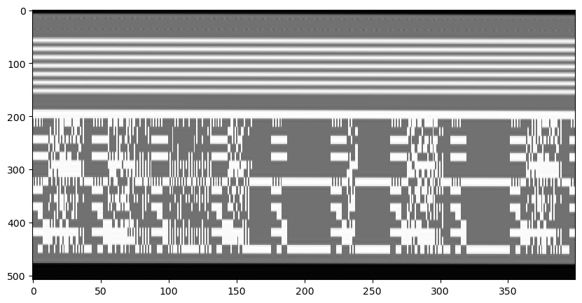
we get the following waterfall.
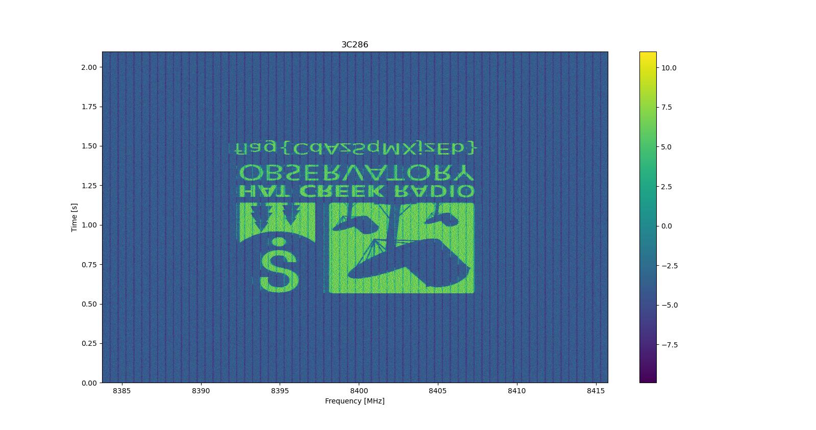
Blame watutil for putting the beginning of the time data at the bottom of the plot. Anyway, it’s possible to read the flag already, or we can simply mirror the image vertically.
Moreover, watutil prints out the following metadata information
--- File Info ---
DIMENSION_LABELS :   ['time' 'feed_id' 'frequency']
        az_start :                              0.0
       data_type :                                1
            fch1 :                      8383.75 MHz
            foff :                      0.03125 MHz
           ibeam :                               -1
      machine_id :                               20
          nbeams :                                1
           nbits :                               32
          nchans :                             1024
            nfpc :                               16
            nifs :                                1
     rawdatafile :   ATA_59839_72460_3C286.0000.raw
     source_name :                            3C286
         src_dej :                      30:30:32.96
         src_raj :                    13:31:08.2881
    telescope_id :                                9
           tsamp :                         0.001024
   tstart (ISOT) :          2022-09-17T17:23:26.000
    tstart (MJD) :                59839.72460648148
        za_start :                              0.0

Num ints in file :                             2048
      File shape :                  (2048, 1, 1024)
--- Selection Info ---
Data selection shape :                  (2048, 1, 1024)
Minimum freq (MHz) :                          8383.75
Maximum freq (MHz) :                       8415.71875
Though not important for the challenge, I took the effort of making the ATA challenges look realistic. Here I put in the metadata for a hypothetical obervation of 3C286 at 8.4 GHz that would have happened at the time I was preparing this challenge.
An alternative way of solving this challenge without knowing anything about filterbank files or blimpy is just using the fact that this is a HDF5 file (the UNIX file command will recognize it as such, for instance). Thus, we can investigate the file using h5py.
In [1]: import h5py

In [2]: f = h5py.File('ATA_59839_72460_3C286.rawspec.0000.h5')

In [3]: f.keys()
Out[3]: <KeysViewHDF5 ['data']>

In [4]: f['data']
Out[4]: <HDF5 dataset "data": shape (2048, 1, 1024), type "<f4">

In [5]: import matplotlib.pyplot as plt

In [6]: plt.imshow(f['data'][:, 0, :]); plt.show()
This would also show the waterfall (and in the correct orientation).
Once the “Filterbank painting” challenge was solved, the “GUPPI painting” challenge appeared. This was basically the same as filterbank painting, except that a GUPPI raw file called ATA_59839_73822_3C286.0000.raw was given instead of the filterbank file. The file had the characteristics as the GUPPI file that I used to produce the HDF5 filterbank file from the previous challenge, which was supposed to be a stepping stone to this one. The way I thought that this challenge would be solved was to use rawspec to produce a new filterbank file, and then plot the waterfall as in the previous challenge. To do this, it is necessary to guess some more or less correct FFT size and averaging, or otherwise the waterfall would look awful. The filterbank file from the previous challenge could provide a reference, but I think that trial and error was also a good and quick approach.
Unfortunately, rawspec can only run using CUDA, so it needs an NVIDIA GPU. I only realized this during the CTF when some people asked me about it. I’m sorry for this, since it makes the work more difficult to people without access to the appropriate hardware (specially taking into account that the in-person attendees would most likely be carrying laptops without an NVIDIA GPU).
I don’t know of a tool that is like rawspec but using the CPU. I think this might not exist, which is unfortunate. On Thursday, which was the last day of the CTF, Lugi Cruz and Sebastian Obernberger, who are interns at the ATA, presented a talk called “Using Allen Telescope Array Data on GNU Radio“. In this talk, they presented gr-teleskop, which has a block to read GUPPI files in GNU Radio as if they were a regular IQ file. I knew that they were working on this topic (specifically, in inverting the polyphase filter bank that is used when generating GUPPI files), but I didn’t know that they had something ready to use. This was an interesting find, because it provided a new, CPU-only, way of solving the “GUPPI filterbank” challenge. Simply, read the GUPPI file in GNU Radio with this block, and then do whatever you want to get a waterfall.
Unfortunately, I’ve heard from some people that tried it that gr-teleskop crashed with the GUPPI file from the challenge. This file doesn’t have the same format as the ones generated by the ATA beamformer pipeline (different number of channels and int8 versus float16 samples), but I hear that gr-teleskope should support GUPPI files from different telescopes, so I’ll be taking a look at this more in detail and send an issue or pull request once I see exactly what happens.
An alternative way of solving the challenge was basically doing the same thing as rawspec by hand. It’s possible to read the GUPPI file either with blimpy or by hand (since the block structure is not that complicated), and then to do the FFT processing by hand on each coarse channel to produce a waterfall (if the GUPPI file samples are extracted to a 2D numpy array, this can be done in one go with np.fft.fft). However, this was too much work for what I intended to be an easy challenge.
The challenge could be solved by running
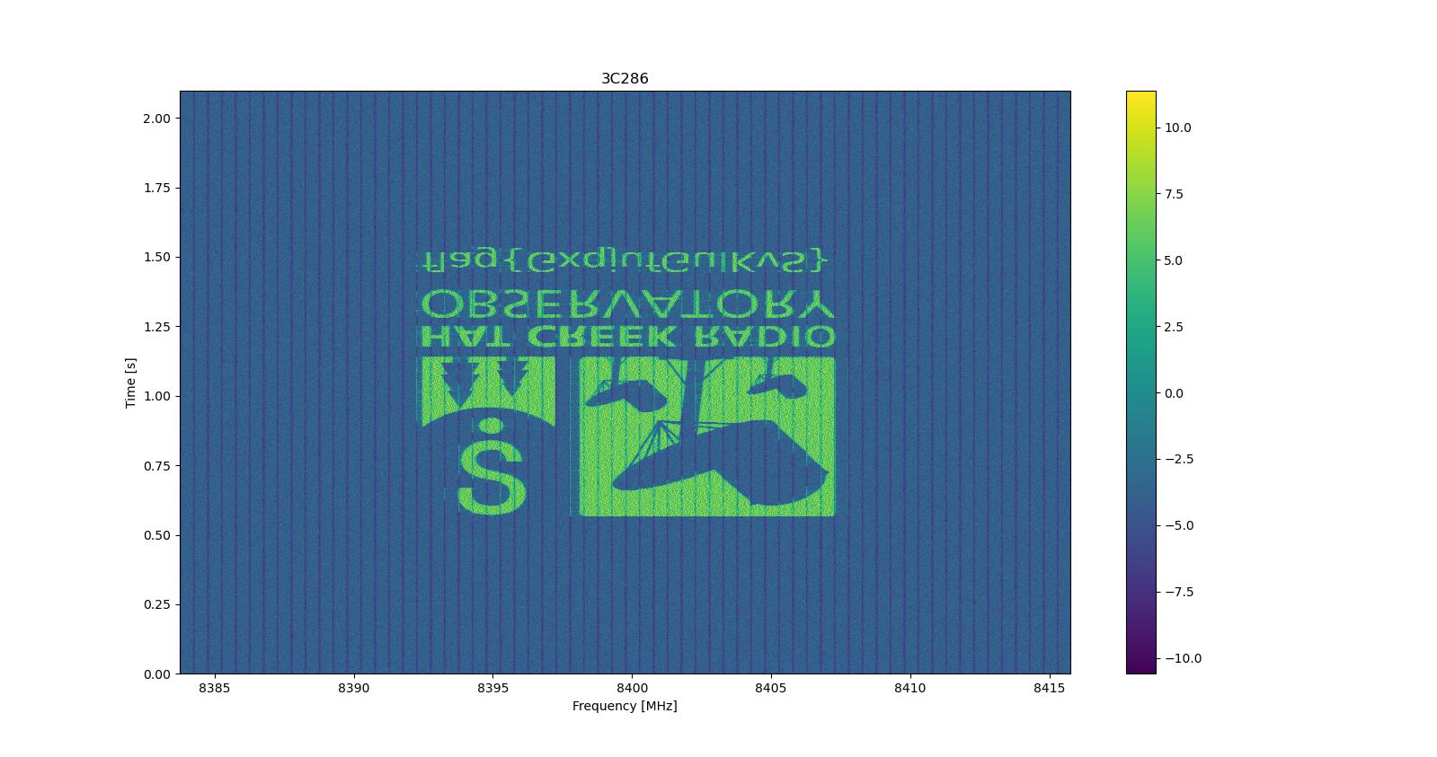
$ rawspec -j -f 16 -t 32 ATA_59839_73822_3C286
$ watutil -p w ATA_59839_73822_3C286.rawspec.0000.h5
This would give the following waterfall, which is the same as the one for filterbank painting, but with a different flag.
The headers for the GUPPI file provide another clue. Since the headers are ASCII text interleaved with the sample data blocks, it was easy to look at these. The header contents were:
BACKEND = 'GUPPI'
TELESCOP = 'ATA'
OBSERVER = 'Daniel Estevez'
SRC_NAME = '3C286'
PROJID = 'GRCON2022 CTF'
RA_STR = '13:31:8.2881'
RA = 202.7845
DEC_STR = '+30:30:32.9600'
DEC = 30.5092
AZ = 91.1149
ZA = 50.4851
STT_SMJD = 63783
STT_IMJD = 59839
STTVALID = 1
OBSFREQ = 8.399750e+03
OBSBW = 3.200000e+01
OBSNCHAN = 64
NPOL = 1
NBITS = 8
TBIN = 2.000000e-06
CHAN_BW = 5.000000e-01
OVERLAP = 0
BLOCSIZE = 134217728
PKTIDX = 0
END
Since I had put my name as “observer”, it was not difficult to look at my blog and find this post about GUPPI files from last month. The post basically contains all the information about how to use watutil and rawspec, and also about how the files for the challenge were generated.
Filterbank painting and GUPPI painting: making-of
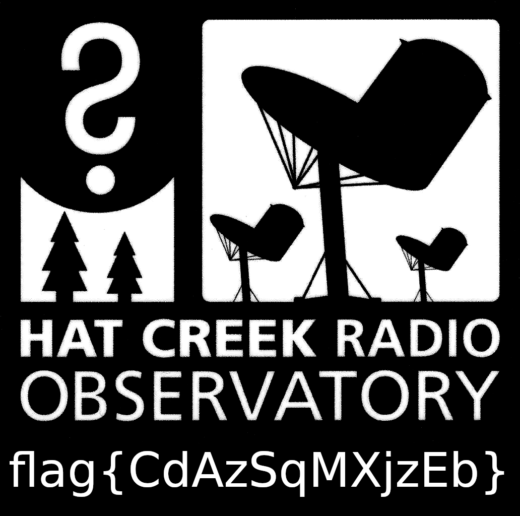
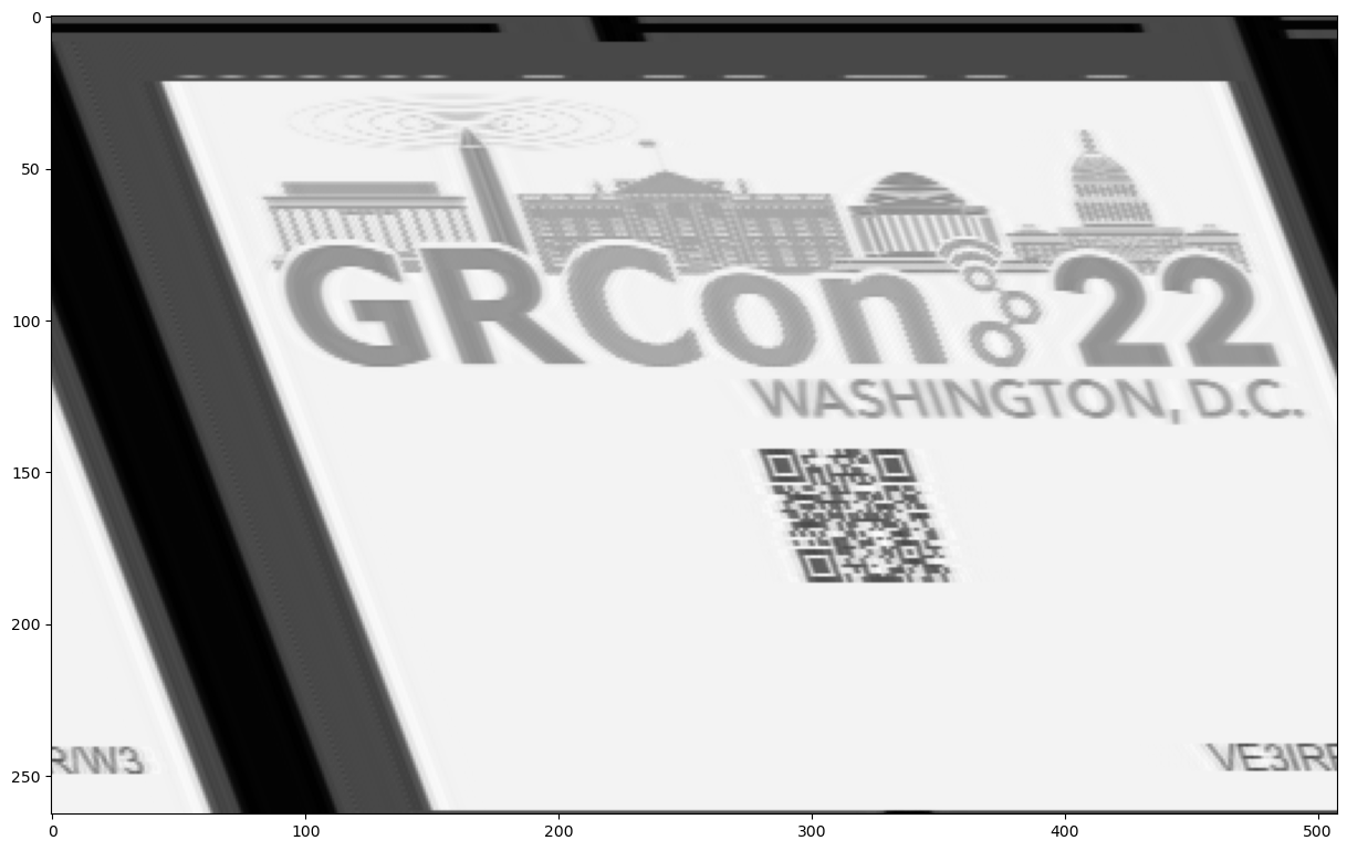
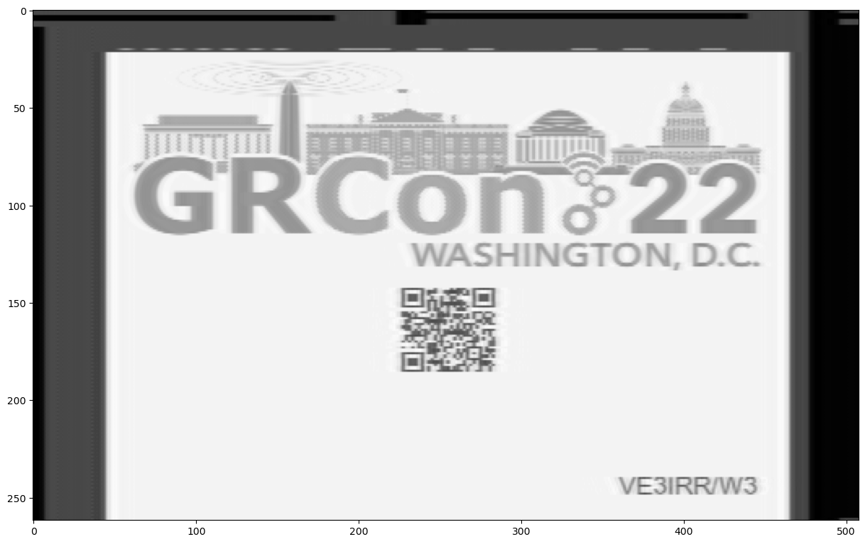
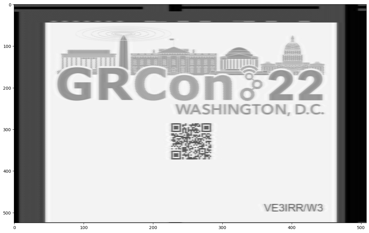
The challenge making-of started with some images like this that I prepared in GIMP. The ATA graphics are actually scanned from a sticker that I brought from my visit to the telescope in July.
The waterfall painting was done with some simple Python code that I wrote in a Jupyter notebook. Basically, it does OFDM with constellation points with random phase, and amplitude given by the image pixels brightness. I also included some AWGN. The output of this Python code was a complex64 IQ file.
Then I used the example flowgraph from gr-guppi to generate GUPPI raw files. I used the same sample rate and polyphase filterbank as in the example, and only edited the metadata. I used Stellarium to calculate the sky coordinates for 3C286 at the time that I was pretending to do the observation.
For the “Filterbank painting” challenge, I took the GUPPI file and converted it to HDF5 filterbank with
$ rawspec -j -f 16 -t 32 ATA_59839_72460_3C286
SETI: discussion
This is my favourite challenge, because I put so much thinking in preparing it and I think it is really cool. I took care to fill it with many little details that probably no one would notice and that don’t really matter for the challenge.
The challenge is intended as tribute to the novel Contact, by Carl Sagan (and also the film). This book/film occupies a very special place in the SETI and radioastronomy communities. I’ve heard from several people that this was one of the things that moved them to study astronomy, and the character of Ellie Arroway is said to be inspired by real-life Jill Tarter, who is one of the most important persons in SETI. An important portion of the book revolves around the analysis of an RF signal of extraterrestrial origin. Therefore, I thought that the topic would be extremely fitting for an ATA track at the GRCon CTF. Alas we can’t play the same trick next year.
While preparing the challenge, I reviewed the book’s plot summary in Wikipedia and some sections of the book itself. I intended to generate a signal as accurate as possible to what the book describes. My thinking was that someone who remembered the book/film could use the plot as a guide for the challenge, and people unfamiliar with it could read up and find the information. I made a few changes and took some liberties that I saw fitted the challenge better. While Sagan describes many details about the signal in the book, I think he never needed to put everything together and actually generate the signal, so not all of what he says necessarily makes sense (more on this below). Also, since this is a CTF challenge, there are some constraints regarding difficulty, file size, etc.
The part of the novel that is relevant to the challenge goes more or less as follows. Scientists participating in a SETI search discover a signal coming from Vega. The signal frequency is 9.24176684 GHz, and its bandwidth is ~430 Hz. It is ASK modulated, with power spectral densities of 174 and 179 Jy. The modulation encodes the sequence of prime numbers in binary. Afterwards they discover the same kind of signal being broadcast from Vega in many frequencies along the RF spectrum.
At some point, the scientists notice that the signal uses polarization modulation. It is described to change between left and right handed circular polarization, thus encoding another message. In fact, when the book first describes the signal, it states that it is linearly polarized, which is another of its noteworthy features, because most signals of astronomical origin are unpolarized or only slightly polarized (with polarization degrees of up to ~10%). The strict reading of this is that the signal is elliptically polarized, with a large axial ratio (so at first glance it looks like linear polarization), and that the sense of the elliptical polarization keeps changing between right-handed and left-handed.
The background here is that for some reason (which may become more clear below) our civilization does not use polarization modulation to encode data (but we use polarization to separate two waveforms, doubling the capacity of an RF link, or to give propagation diversity). However, an alien civilization may as well use polarization modulation, as it’s just another property of the RF wave that can be manipulated to convey information. Thus, the presence polarization modulation wasn’t obvious immediately.
The polarization modulation sends a binary sequence (the two symbols are right-handed polarization and left-handed polarization), and the scientists see that it repeats with a period on the order of \(10^{10}\) that is the product of three distinct prime numbers. They decide to arrange the sequence as a 3D array (there are only 3! = 6 possible ways to do this, given that the length is a product of three distinct primes), and interpret it as video. Note that this must be black-and-white video (not grayscale!), in the sense that pixels are either black or white. An “gray interpolation filter” is mentioned, which makes a lot of sense if the video uses dithering. There is also an audio track to go with the video on an “auxiliary sideband channel”, but no more details of this are given.
The video turns out to be Adolf Hitler opening the 1936 Olympic Games. The plot then continues explaining that this was the first powerful enough radio transmission to reach nearby stars, and the aliens are just playing it back to us as a sort of “we’ve received you” message. The signal happens to be received at Earth after the round-trip light-time to Vega (50 years) has passed after the Olympic Games. Upon further analysis, the signal is revealed to contain detailed plans for an advanced machine, and so on, but here ends the segment of the book on which my challenge is based.
The hardest part of setting up this challenge was making sense of this polarization modulation thing. It may work very well as a device for the novel plot, but it also needs to work well when you do try to deploy it as a real RF communications technique, as well as be an interesting trick for the CTF challenge (where the main goal was to make people read up a bit more about polarization, since most people are not too familiar with it).
So, polarization modulation is a weird concept. Let us toy with the idea of changing the polarization of a CW carrier between two polarization states to transmit bits. The first remark is that in general we are going to see the polarization changes as amplitude changes in our receiver. For example, we could have a horizontally polarized receiver, and the signal changing between horizontal and vertical polarizations. To our receiver, the signal will appear when it is horizontal, and disappear when it is vertical. If we have a dual polarization (horizontal and vertical) receiver, as is common in radio astronomy, the signal will pop up in one polarization channel, and then in the other.
This is no fun for the CTF, because if polarization changes appear as amplitude changes, then people can completely skip dealing with the polarization and treat the signal as ASK. Luckily, there are some choices of polarizations for which we do not see amplitude changes. These depend on the polarization of the receiver.
The ATA feeds are linearly polarized, with channels called X and Y, which are horizontal and vertical (or the other way around; I never remember). For this kind of receiver, there are two choices of two orthogonal polarizations for which the X and Y channels see the same amplitude:
- Diagonal linear polarizations, at +45 and -45 degrees.
- Right-handed and left-handed circular polarization (RHCP and LHCP).
I don’t like the idea of diagonal polarizations, because it looks like “wow, what a coincidence!”. In space there is no absolute frame of reference for what is vertical and what is horizontal, so the chances that the aliens are sending an RF signal that is polarized at a perfect 45 degree angel relative to our feeds are slim (specially taking into account parallactic angle rotation). On the other hand, circular polarization works very well, because it is not affected in this way by geometric rotations. This is the reason why circular polarization is very popular for space communications. Besides, the book says that the polarization modulation uses circular polarization.
So let’s think that we want to make our CW carrier change between RHCP and LHCP. In our X and Y channels, circular polarization is manifested by the phase offset between X and Y: there is a phase offset of 90 degrees for RHCP and of -90 degrees for LHCP (or the other way around, depending on your handness conventions). So if we want the CW carrier to switch, say from RCHP to LHCP, the phase difference between the X and Y channels must change by 180 degrees. To do so, we either maintain the phase of the signal in one of the channels and make the phase in the other channel jump by 180 degrees, or we make the phase of both channels jump simultaneously so that they end up changing their phase difference by 180 degrees. In any case, there must be a phase jump in at least one of the channels.
So this is a problem for the CTF, because our polarization modulation appears as phase modulation. In fact, unless we randomize the phase jumps that need to happen, people will be able to read off the data from the phase modulation, defeating our whole scheme. The idea of randomizing the phase jumps is silly. No one would realistically do that as a communications scheme. I guess that in reality how the phase jumps look like depends on how the RHCP and LHCP polarizations are physically generated. But what needs to happen is that if we go RHCP, then LHCP, then RHCP, first the phases in the X and Y channels start at some values, then change to some other values for the LHCP, and then they must change back to the same initial values for the RCHP. In this case it’s perfectly possible to read the data as phase modulation in a single channel, despite the fact that the two constellation symbols will not be 180 degrees apart in general.
So it appears that our idea to do polarization modulation by changing between RHCP and LHCP doesn’t work very well (the same problem with the phases happens if we try to use diagonal polarizations). Luckily we are saved by the concept of fractional polarization.
It happens that a coherent waveform, such as our CW carrier, or basically any of the waveforms we use in RF communications, can only have a pure polarization (either linear, circular, or elliptical). However, an incoherent waveform, which is basically Gaussian noise, can be unpolarized, or have any degree of polarization between 0% and 100% (this indicates the fraction of the total power that is polarized). The polarization is measured using something called Stokes parameters, which essentially involve measuring average power on different polarization channels, such as X and Y. Therefore, for a noise-like signal, its polarization is not an instantaneous property, but something that must be measured over some time average. (I should point out that here I am using the terms coherent vs. incoherent rather loosely; the Wikipedia article about unpolarized and partially polarized light treats these topics in more detail).
If we use a polarized noise-like signal, instead of being able to choose between two values, RHCP and LHCP, we have a continuum range: from purely RHCP on one extreme, passing through unpolarized in the middle, and finishing at purely LHCP. This is nice, because if we want to send images we can encode pixel brightness as an analog value, instead of only black or white. What is more important is that for this noise-like signal it is not possible to see the polarization changes as phase jumps, since the idea of measuring the phase of random noise doesn’t even make much sense.
A pragmatic way to think about the trick we have found is that to disguise the phase changes that need to happen between the X and Y channels when the polarization changes is to make the phase of our signal change all the time. This makes our signal be random noise.
Now we may ask, does this idea look like a reasonable communications method? Well, since spark gaps fell out of use, all our RF communications have been coherent (in the sense I’m using here; I’m completely aware of non-coherent demodulation methods), because it is perfectly possible to build RF oscillators that generate a clean, coherent, sinusoid.
On the other hand, my understanding is that many kinds of optical communications happen with an incoherent light source (also known as broadband light source), because it’s not easy to build coherent optical oscillators. I don’t know much about optical communications, but I think that even lasers have a noticeable linewidth. For this reason, incoherent light sources are typically modulated in amplitude, since phase or frequency modulation don’t make sense for such a noise-like source. So the point I’m trying to get at is that for communications, coherent signals are more useful, but sometimes it is not possible to build clean enough oscillators that can support them.
Now, all known natural astronomical sources emit incoherent radiation. Think of many electrons doing their own random things in a magnetic field (synchrotron radiation). Each of them gives a small, random contribution to the total waveform. Polarization in these astronomical sources (either linear or circular) arises because of the presence of magnetic fields. These natural sources radiate tremendous amounts of RF energy. They involve huge areas of space, large amounts of matter, or whatever.
Now imagine some advanced civilization that has some ability to create or control these kinds of natural astronomical sources, and to manipulate their magnetic fields to vary the polarization. Then it might make sense for them to use these kinds of sources as interstellar communications beacons, simply because they can get out so much more power than with clean electronic oscillators and amplifiers (and the power comes off omnidirectionally, which may be useful). For this kind of sources the only possible modulation methods that come to mind are amplitude and polarization, and I don’t know how they could achieve amplitude modulation, so perhaps polarization modulation seems the most reasonable option.
There are surely many loose ends with this reasoning, but anyway, this is a CTF, not a SETI research paper. Hopefully I’ve managed to convince that my idea of a noise signal with polarization modulation is not too far fetched as a communications mechanism.
With the idea of doing polarization modulation on a noise signal set in mind, I then decided to encode a single image as analog slow-scan television. I find that the idea of encoding an image as a sequence whose length is a product of two primes is not very good, neither for a CTF nor for active SETI (though this was used for the Arecibo message). First, the idea of the receiver determining the length of the sequence because they observe the same sequence repeating is not too robust to corruption by noise. Second, because in practice the receiver will typically attempt to compute the autocorrelation of the received data and look for peaks. With this, the receiver will certainly find the period of the sequence, but they will also find the correlation peaks given by the line length (see the solution to the challenge below).
Including a nice blanking interval in the analog image signal will ensure strong autocorrelation peaks that the receiver will detect and become interested in. Certainly, one of the things I try first when reverse engineering signals (even streams of digital symbols) is to compute and plot the autocorrelation, and to represent the data as a matrix with a line length corresponding to the autocorrelation peak lags. This is a much more fruitful and robust technique than trying to notice that the length of some piece of data is some particular number.
Interestingly, one of the challenges of the CTF, “Solve my bomb; Part 1: Bounty” was done like Arecibo message. There was a hint about images being sent line by line, and the image was sent as 0’s and 1’s in FSK using a semiprime length. When I got the hint, I immediately thought slow-scan television. I took the FSK signal as analog FM, found the line length via autocorrelation, and plotted the image. I never noticed that it was digital rather than analog, that there was a symbol rate, and that the message was some particular size.
Finally, I decided to send a single image rather than video because a single image was enough to contain the flag, easier to decode, and produced a smaller file. Indeed, there is no way I could have included in a reasonable file size the \(10^{10}\) bits of information they state in the book. This is another implausible aspect of the book, because if you think about it, binary polarization modulation is not magic and still has a spectral density of 1 bit/Hz, so with a waveform that is 400 Hz wide it would take 289 days to send \(10^{10}\) bits (on the other hand, this \(10^{10}\) value corresponds to 424 seconds of 1024×768 black and white (not grayscale) raw video at 30 fps, so it’s a reasonable value for the novel).
SETI: solution
Certainly I didn’t expect the CTF participants to go through all the thinking I have described above. I intended people to get the references to Contact, think of looking at the circular polarization, discover that there is actually a signal there, think again of the book/film, and try to get an image or video out of there. For this, the main difficulty was plotting the data with a line length that is not too far off from the correct one. Once you do that you can already see some geometric patterns and refine the line length by hand.
An autocorrelation of the polarization signal was the easiest way to find the line length. I think that maybe it’s possible to look at the time domain polarization signal and discover that there is some periodicity, and thus arrive at the correct line length (specially because of the large blanking interval I put and because the image is not too busy, and the background is monochrome). However, to do this it is important to average the polarization with the correct length. Too short of a length, and it will be too noisy to notice anything (recall that the polarization of a noise signal is only defined as a time average). Too long of a length and you’ll average multiple lines together.
The challenge description said:
Last Sunday we received an unusual signal during a routine observation with the Allen Telescope Array 20-antenna beamformer. Experts believe that the signal originates from outside the solar system.
The “last Sunday” part was intended to give a sense of urgency and novelty. The way this story is told is that the ATA scientists have found an extraterrestrial signal on Sunday, but since they’re not able to understand it completely, and coincidentally GRCon starts next day, they’re dropping the recording as a CTF challenge. Surely one of the participants will manage to solve the mystery (unfortunately no one did).
Two SigMF files, ATA_59848_08825_HIP91262_polX and ATA_59848_08825_HIP91262_polY were given. The SigMF description says “HIP91262 ATA 20-antenna beamformer polarization X (GRCon22 CTF)”, and gives a timestamp of 2022-09-26T02:07:05Z and a frequency of 5.681361 GHz (below I’ll explain why I decided this not to be 9.2 GHz as in the book). The sample rate is 6 ksps. Note that the filename has nearly the same invented, but realistic looking, format that I used for the filterbank and GUPPI painting challenges. I don’t expect anyone to know what HIP91262 is, but a quick Google search shows it’s the star Vega. Since we are given files for polarization X and Y, it might already be suspicious that the polarization has something to do with the challenge.
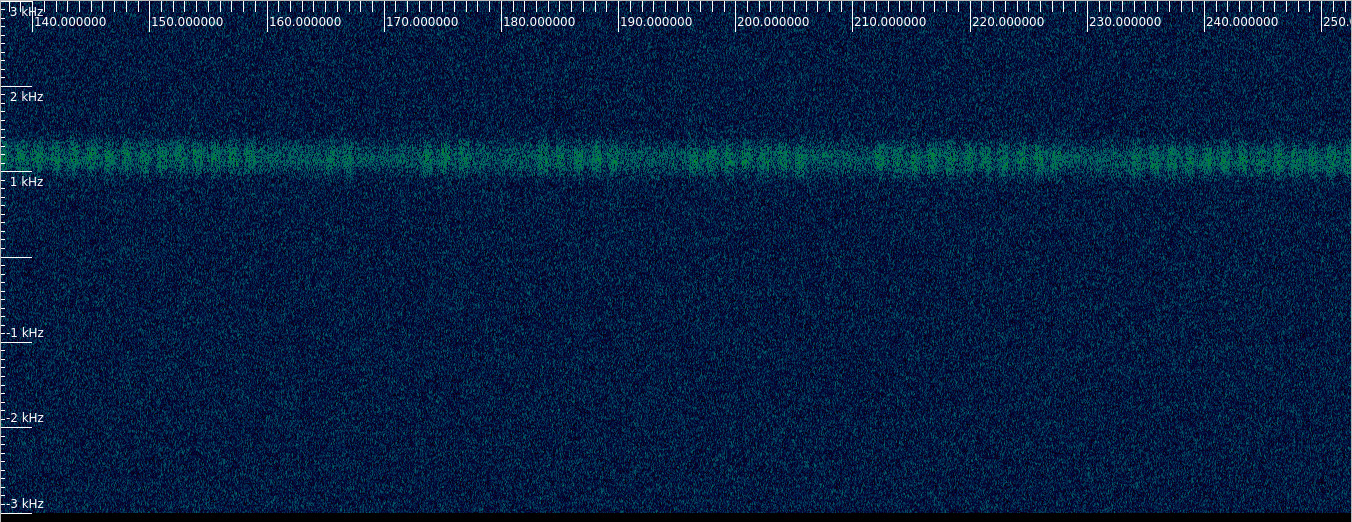
If we look at the waterfall we immediately notice some pulses in the signal, and a break in the pulses. This is the waterfall for polarization X, but polarization Y looks exactly the same.
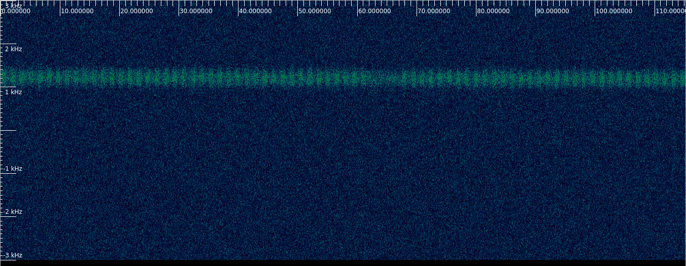
The file is quite long (1 hour), so it is reasonable to continue looking and move in time. We note that the signal Doppler drifts down, which is fair, because a signal from Vega should drift down because of Earth rotation Doppler.
We quickly arrive at a part where we can see 2 pulses, then 3 pulses, then 5, then 7. If we count the next pulse trains we see 11 pulses, 13 pulses, etc. These are the prime numbers.
Here I have deviated from the book and encoded the numbers in unary base rather than binary base. I think this makes way easier to see that these are prime numbers. The problem with binary is that you need a way to separate the numbers, and there is also the issue of endianness. Unary really stands out on its own. I think that counting (pulses in this case) is a much more basic ability than binary encoding, so maybe the aliens in the book should have also used unary.
I have also increased the relative power difference between the pulse and no-pulse power levels from what the book says. The difference between 174 and 179 Jy is only 0.12 dB, so it’s quite hard to notice. I wanted the pulses to stand out easily.
So at this point we have a series of prime numbers coming from Vega, so I hoped the reference to Contact to come to mind or pop up from a Google search (later on during the CTF, since no one had solved the challenge yet, I just dropped the reference to Contact on the CTF chat as a hint to try to help people). Once it is clear that the key is in the polarization, the idea to look at the circular polarization in particular comes either from the book or from the obervation that since the two files are linear polarization (X and Y), and they look identical in the waterfall, we’re already looking at the linear polarization and see nothing relevant there.
There are basically two ways of measuring the circular polarization (i.e., the Stokes V parameter) using GNU Radio if we are given signals in the X and Y polarizations. The first involves converting to RHCP and LHCP as \(R = X + iY\), \(L = X – iY\), and then computing the difference in power of these. The second involves computing \(\operatorname{Im}(X \overline{Y})\). If you work out the math you’ll see that these two ways give exactly the same result, except perhaps for the sign (I’m completely ignoring signs and handness conventions, since we don’t care about them to get a video signal).
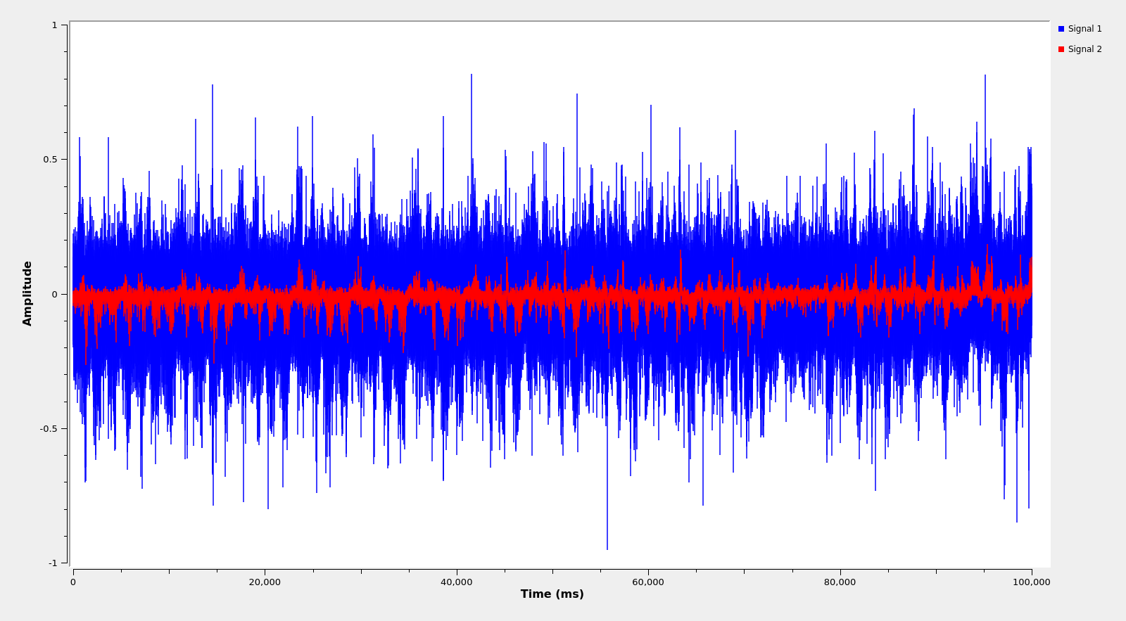
If we do any of these and plot the Stokes V in the time domain, we already see that there is something going on, but the signal is too noisy. It is reasonable to try a lowpass filter. Below I show the unfiltered signal in blue, and the signal filtered through a 100 Hz lowpass in red.
In doing this, I’m being a bit lazy and going for the most direct way to the solution, so I’m processing the full 6 kHz bandwidth, which includes the signal and the noise. This is not the best idea. Probably it pays off to perform Doppler correction and lowpass filter the signal before doing anything. An easy way to do Doppler correction is with my Doppler correction block. The Doppler is almost linear versus time, so we can measure in the waterfall the Doppler at the beginning (~1250 Hz) and end (~-200 Hz) of the IQ file and then write a Doppler file that lists these:
0 1250
3600 -200
If we do this, probably we will already get something in the Stokes V that looks like the red trace above, because we would be applying a lowpass filter with a cutoff somewhere between 200 Hz to 300 Hz (the signal bandwidth is around 400 Hz, as in the book).
The following GNU Radio flowgraph shows the two ways of computing the Stokes V and the output to files. There is also a part on the bottom to which we will come back later.
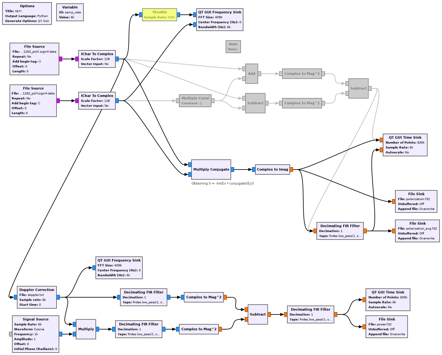
We can investigate the time domain Stokes V signal using Python. I prefer that to using GNU Radio, since GNU Radio doesn’t provide good tools to plot the autocorrelation, select peaks, etc. I will use the unfiltered signal (the one in blue in the plot above), just to show that it isn’t necessary to apply filtering to solve the challenge. One of the beauties of analog video is that even if it’s very noisy, we are able to recognize features in the image. The Jupyter notebook for this part can be found here.
If we plot the autocorrelation we get the following.
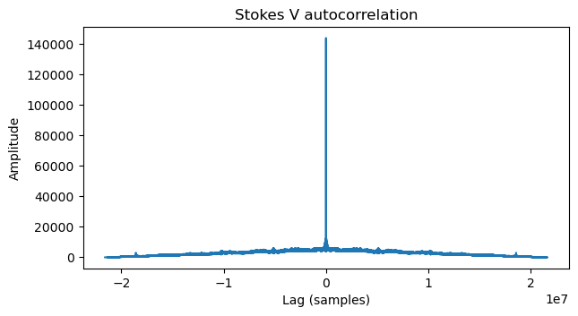
Since the autocorrelation of any signal is very strong at a lag of zero, and the autocorrelation is symmetric, it is reasonable to plot only the right half of this plot, omitting lags very close to zero, so that the vertical scale lets us see the peaks at non-zero lags better. This is shown below.
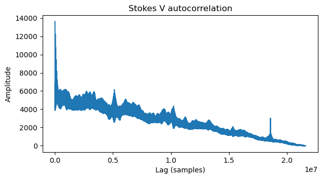
We see that there are a few peaks. In particular, a noticeable peak is near the right part of the plot, at a lag of around 1.8e7 samples. This in fact corresponds to the total length of the image. It takes somewhat less than 1 hour (which is the length of the IQ file) to transmit the image, so part of the image repeats, and this is what this peak is showing.
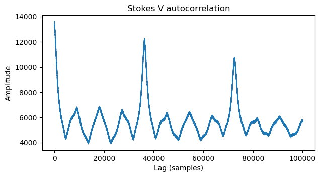
If we think for a second about what we want to find, which is the line length of the video transmission, none of the peaks that we see in the plot above are relevant. The video image should have hundreds or thousands of lines, so the autocorrelation peak given by the line length should be at a 1/100 or 1/1000 of the total file length. The peaks above are at much larger fractions of the file length, and so must correspond to larger features in the image that encompass many lines. To find the line length we need to look at the lags close to zero.
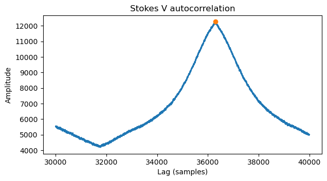
We do so, obtaining the plot below. There is a noticeable peak at ~37000 samples. A peak at twice this lag is also present, and there are smaller peaks that seem to be at multiples of 1/4 of this value. We decide to go for the peak at ~37000 samples.
We find the exact location of the maximum of this peak and take that as the line length.
We reshape the Stokes V time domain data as a matrix using this line length and plot it. The image is shown below. The contrast is not great, because it is chosen automatically, but we can already see a vertical bar, some geometric features, and what looks like text on the right. The vertical bar is slightly slanted, so we tweak manually the line length to make it straight. This vertical bar corresponds to the blanking interval that I put in the video signal.

The nice thing about this approach is that it is tolerant to mistakes in the line length. For instance, if we had used twice the correct line length, we would get a doubled image, and we would notice and halve the line length. If we had used half the correct line length, then we would still see the image, but would get a different thing on even and odd lines, such as when video interlacing is messed up. We could then try doubling the line length. Values which are close to the correct ones give slanted images, and can also be corrected by hand. However, values that are too far off give a complete mess with no clues of how to fix it.
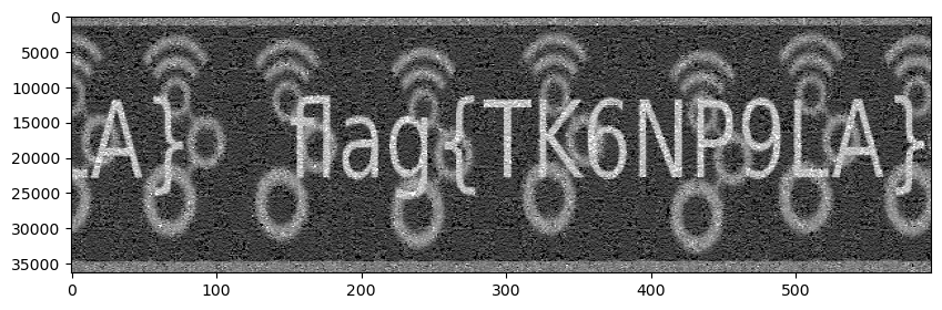
After tweaking the line length by hand (only by 3 samples) to make the vertical bar straight, rotating the image, changing the aspect, increasing the contrast, and circularly shifting the matrix to put the text in the middle (and the bar at the top and bottom), we get the following.
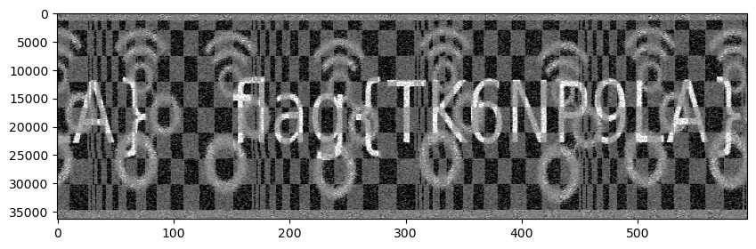
We can clearly see the flag, and the GNU Radio logo. The reason why we have had to rotate the image is because I decided make the video lines of this image be scanned vertically rather than horizontally. All the video systems that I know of scan horizontally, so I decided to include this twist for fun (it is very easy to sort out for anyone that manages to see the image). Incidentally, the book mentions “And try rotating it about ninety degrees counterclockwise” when discussing how to display the video. An existing system that scans vertically is Hellschreiber, and in some sense this video transmission is similar to Hellschreiber, because it is sending an image which is a line of text, so its width is much larger than its height.
With this, the challenge is solved, but there remains a question: what is the chequerboard pattern that appears on the image? This is actually caused by the ASK pulses that encode the prime numbers. Since we are plotting the power of the signal that is circularly polarized, power changes caused by the ASK modulation are registered in the image (the ASK modulation is applied to the partially polarized noise signal as a whole, increasing its total power and not changing the polarization degree).
As we will see in the making-of below, there are exactly 8 ASK symbols (either pulse or no-pulse) in the time it takes to send a line of the image. Thus, the pulses on adjacent lines get lined up in the image and appear as rectangles. The gaps between the primes consist of an even number of no-pulse symbols (whereas between pulses in the same prime we only have gaps of one no-pulse symbol). Thus, every time that the signal moves on to a new prime, the pattern of pulse/no-pulse gets offset by one symbol, and this is what causes the chequerboard pattern. The width of the chequerboard rectangles is thus proportional to the number of pulses that are in the prime number, so we see that the width increases as the signal keeps sending larger and larger primes, and then goes back to very narrow when the signal starts again with 2, 3, 5, 7, 11, etc.
I could have prevented the chequerboard pattern from showing up in the image simply by making the extra power of the ASK pulses be unpolarized, so that the Stokes V parameter is not affected by the presence of the pulses. However, I decided that it was more natural to have a signal where the ASK modulation affects the polarized signal as a whole, rather than adding more unpolarized power, and that perhaps the chequerboard pattern could help someone find the correct line length by providing another simple geometric pattern on the image.
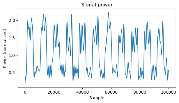
The way to remove the chequerboard pattern is to normalize the Stokes V by dividing by the total power of the signal (which is called Stokes I). Since the signal has the same power in the X and Y channels, we can simply measure the power in the X channel. I have included the power measurement in the bottom of the GNU Radio flowgraph. To do this, the Doppler of the signal is corrected, a lowpass filter with a cutoff frequency of 300 Hz is a applied, and signal plus noise power is measured. The same is done on another part of the spectrum to measure noise power alone and subtract. The power measurement is averaged with a lowpass filter with a cutoff frequency of 5 Hz.
The beginning of the signal power is shown here. We can see the ASK pulses, even though the power measurement is somewhat noisy. The power has already been normalized so that the average power is one.
We can now divide the Stokes V measurement by the power measurement. To do so, it is important to take into account the group delays of the lowpass filters that we have used everywhere, as otherwise the measurements won’t line up correctly. This gives the following image, where the chequerboard patter has disappeared.
If instead of using the unfiltered Stokes V measurement we start off with the filtered Stokes V mesurement, we get the image below. We see that the difference in image quality is very small, so averaging the Stokes V is not really necessary. The main reason is that in any case matplotlib is doing some averaging to rescale and display the image, as it is more than 35000 pixels (samples) high.

SETI: making-of
Since I tried to make my Allen Telescope Array challenges as realistic as possible, I chose a timestamp for the observation when Vega was high up in the sky at the telescope. I intended to calculate and include the correct Doppler shift for Vega, and I wanted the Doppler drift to be clearly visible in the waterfall. For this, the signal should be narrower than the total Doppler drift along the IQ file.
The Earth rotation Doppler drift is maximum when the star is higher up in the sky, and it is also reasonable to conduct observations at this time to reduce atmospheric noise and losses. I calculated that for microwave frequencies the Doppler would change on the order of 1 kHz in one hour, so having a signal that was a few hundred Hz wide as in the book was good to make the Doppler drift easily visible.
Since I needed to generate many frequencies to construct the waveform (the carrier frequency, the pixel duration, the line length, the ASK pulse duration, etc.), I decided to make everything a suitable power of two multiplied by the HI line frequency of 1420.406 MHz. This was intended just as a subtle reference to the importance of this frequency in radioastronomy. It was unimportant for the challenge, and I doubted that anyone would notice, specially because of Doppler. I would apply Doppler to all of the waveform features, not only the carrier frequency, just as it would happen in real life.
All the signal generation is done in this Jupyer notebook. I used Astropy to calculate the Doppler from Vega using the heliocentric radial velocity correction. This accounts for Earth’s rotation and motion around the Sun, but not for the relative motion between the Sun and Vega. Thus, this Doppler is what we would see if the aliens are Doppler correcting their transmissions for a zero Doppler reception at the Sun. If they are beaming towards the solar system, that looks like a reasonable thing for them to do. The radial velocity comes out to 13.8 km/s, which means that all the frequencies involved in the waveform will change by about 46 ppm. The bulk of this velocity is due to the Earth motion around the Sun. On top of that we have the Earth rotation Doppler, which changes noticeably throughout the course of the observation.

Following my idea of making all the frequencies a power of two times the HI line frequency, the best choice for the carrier frequency was 4 times the HI line frequency, which gives nearly 5681.623 MHz. This is good, because it is a reasonable frequency for the ATA to observe at, and is also relatively high, giving more Doppler drift in the waterfall. If we had chosen 8 times the HI line frequency, we would have obtained 11363 MHz, which is a bit high for the ATA. The ATA feeds do cover this frequency, but observations are usually conducted at lower frequencies, and also 11.3 GHz is full of RFI coming from satellite TV GEO satellites. This is the reason why the signal for this challenge sits at 5.7 GHz rather than 9.2 GHz as in the book. I felt that this was a small liberty I could take, specially because the book says that copies of the signal were broadcast all over the spectrum. The only special thing about the 9.2 GHz signal is that it’s the one that they found first.
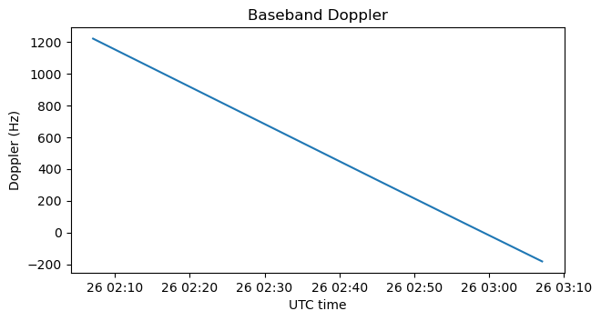
The Doppler at 5.7 GHz is quite large, on the order of -260 kHz. Since I wanted to make the sampling rate of the IQ file small in order to reduce its size, I chose the centre frequency accordingly. A frequency of 5681.361 MHz centres the received signal more or less well at baseband, so this is the centre frequency that I chose for the IQ file.
Here we see the Doppler frequency at baseband, once we take the centre frequency into account. This is what appears on the IQ file.
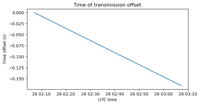
The Doppler is applied to the remaining features of the waveform using the concept of time of transmission offset. Since according to the Doppler Vega is receding from Earth, the time of flight of the signal increases with time. We can express this as the offset in the time of transmission that we see in the signal at each reception time, compared to the time of transmission that a signal with no Doppler would have had. This is just the integral of the radial velocity in units of time.
In order to keep the file size reasonable small, I decided to make the IQ recording one hour long. We need to be able to fit a whole image in that duration. The signal bandwidth is going to be some 400 Hz, as in the book, but as I mentioned, the measurement of Stokes parameters needs some averaging. Therefore, for best results the pixel clock should be much smaller than the signal bandwidth. This means that the image will be sent pretty slowly. I decided a pixel frequency of \(2^{-26}\) times the HI line frequency, which gives 21.17 Hz. At this rate, a 256 x 256 image (a reasonable minimum size to draw a flag as text) would be sent in 0.86 hours.
I prepared the following image in GIMP. I decided to make it 512 x 128 rather than 256 x 256, as that aspect ratio would be more convenient for writing the flag as text. Grayscale values will be encoded with different circular polarization values. Pure white is pure RHCP and pure black is pure LHCP (or the other way around). I also put in a thick bar of 50% grey (corresponding to unpolarized) to be used as blanking interval, in order to simplify finding the appropriate line duration. As I mentioned above, the image is scanned using vertical lines rather than horizontal lines by the slow-scan TV signal.
The noise signal encoding the image is constructed in the following way. Each pixel will be formed by 64 “symbols” which are uncorrelated normal random variables. Thus, these symbols give white Gaussian noise at 1354.6 sps. A filter will be applied to this to reduce the bandwidth of the noise to approximately 400 Hz and to obtain the final sample rate of 6 ksps. Symbols are generated for the RHCP and LHCP polarizations, using the standard deviations given by the pixel brightnesses to achieve the polarization we want. Then we convert from the RHCP and LHCP basis to the X and Y basis, and work with the X and Y channels from this point on.
Now we apply the ASK modulation which contains the prime numbers. I decided that a pulse frequency on the order of 1 Hz was easily visible in the waterfall for a signal of this bandwidth. It was also easy to hear in case someone tried to listen to the signal. The exact pulse frequency is constructed such that each pulse lasts 1024 of the “Gaussian noise symbols” that we computed. Therefore, a pulse lasts 16 image pixels, so there are 8 pulses per image line.
The sequence of primes consists of only the primes 2, 3, 5, …, 61. In the book the signal is described to count up to very large primes, but I decided to make the sequence relatively short, so that it repeats multiple times times during the recording. My hope was to make clear, and not so difficult to see, that these are the prime numbers, but that there is no message hidden in them for the CTF challenge.
I decided to make the shape of the power spectral density of the signal be a Gaussian, because this looks more “natural” than a root-raised cosine or something like that. To achieve this, I built a polyphase arbitrary resampler using a Gaussian as prototype filter and ran the “Gaussian noise symbols” through it. The parameters of the polyphase resampler (number of arms and taps) were chosen to make the spurious products small enough.
When running the polyphase resampler, we also take into account the time of transmission offset that we calculated previously. In this way, we apply the Doppler to all the signal features, such as the pixel clock, pulse duration, etc. Strictly speaking, we aren’t applying the Doppler to the signal bandwidth. The polyphase resampler maintains the same output power spectral density, while in reality the signal bandwidth should decrease slightly with time, because the Doppler is decreasing. This effect is very small, however, so I didn’t think of including it.
On the other hand, Doppler really affects the slow-scan TV image. If we used the nominal line duration to try to assemble the image, we would get a slanted image, because Doppler has made the line duration longer. However, since the line duration is a weird made up value, I didn’t intend anyone to think about it. While solving the challenge we effectively find the effective line duration, with the Doppler already applied. Interestingly, due to Doppler drift there is also a small curvature in the image. The effect is very small to notice easily, however.
When performing the resampling, a more or less random time offset is also added. This is used to make the IQ file start somewhere in the middle of the transmission of the image and avoid the unrealistic coincidence of having the image start exactly when the observation began. As it happens, the recording started while the second to last character of the flag was being sent, as we can see in the solution.
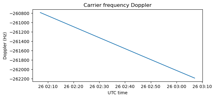
After running the signal through the polyphase resampler, Gaussian noise is added to set the SNR. I adjusted this by hand to make the signal have a moderate SNR. Finally, the carrier frequency Doppler is applied and the IQ data is saved as a SigMF dataset.
As I wanted to erase all traces that I was preparing these files well in advance rather than actually observing with the ATA “last Sunday”, I even removed the file timestamps in the tar file in which I put the two SigMF datasets. I learned how to do this in a StackOverflow answer.
OFDM 101
The other challenge that I submitted was called OFDM 101. This was included in the “Miscellaneous” category. I have been working a lot with LTE this year, and I think that many people have never dealt with OFDM, and there are perhaps fewer good resources to learn about it than for other modulations, making it seem more difficult than it really is. Thus, I thought it would be a good idea to make an OFDM challenge, to get more people interested in learning about OFDM. Perhaps my work on LTE could even provide some useful resources.
Even though I classified this as a difficult challenge, because reverse-engineering a custom OFDM modulation is never going to be as easy as reverse-engineering something like FSK, I tried to make it as simple and straightforward as possible, hence the “101” in the name of the challenge.
My idea was to make the data be ASCII text, which is easily recognizable. I used the text of the Wikipedia article on OFDM as filler text and inserted the flag somewhere in the middle. This had the goal of making the participants demodulate all the data rather than handling only the first few symbols and calling it a day, and providing some randomness for the data to prevent a weird looking waterfall. I think that if you get a bunch of text, the idea to grep for something containing flag{ is obvious.
The OFDM modem was built around a 1024 point FFT, occupying only the central 3/4-ths of the carriers, and using a cyclic prefix of 1/8. The modulation was QPSK. I think these are rather standard values that won’t surprise anyone. The frame structure was formed by frames of 8 symbols, in which the first symbol was all pilots and the 7 remaining symbols carried data. ASCII data was encoded in the QPSK symbols in the most straightforward way: allocating two bits per subcarrier in order of increasing frequency.
The pilot symbols were made by repeating the CCSDS 32-bit syncword 0x1ACFFC1D as many times as necessary to fill all the subcarriers in each of the symbols dedicated to all pilots. Since there are several ways of encoding pairs of bits as a QPSK symbol, I thought that it was appropriate to give the syncword as part of the challenge, to avoid any possible ambiguities in the QPSK encoding. Thus, the challenge description said
0x1ACFFC1D is your friend.
I made a simple Jupyter notebook to generate the OFDM signal without any channel effects. Then I used a GNU Radio flowgraph to add the channel effects. I added AWGN, carrier frequency offset, sampling frequency offset, and dropped a bunch of samples from the beginning, to avoid the IQ file starting exactly at the beginning of the data. I also added a multipath channel with some taps that I chose by hand. The multipath channel didn’t change with time, but I guess this is somewhat realistic because the IQ file was rather short (only 95 milliseconds).
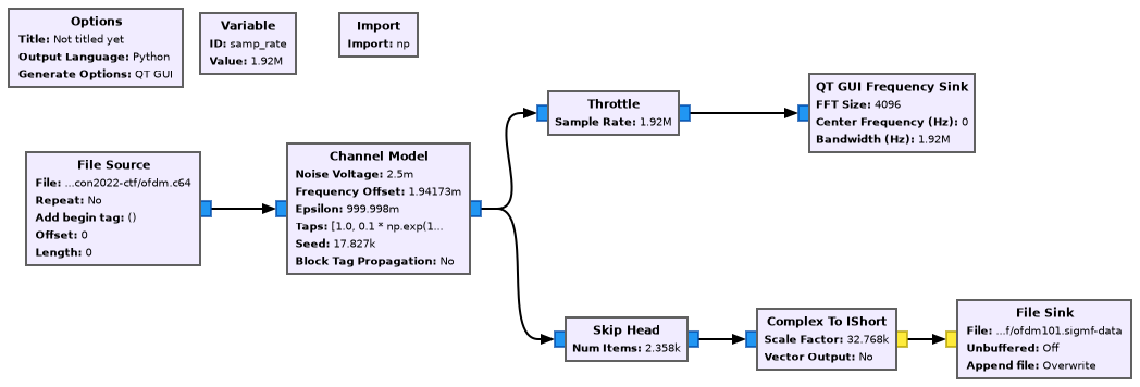
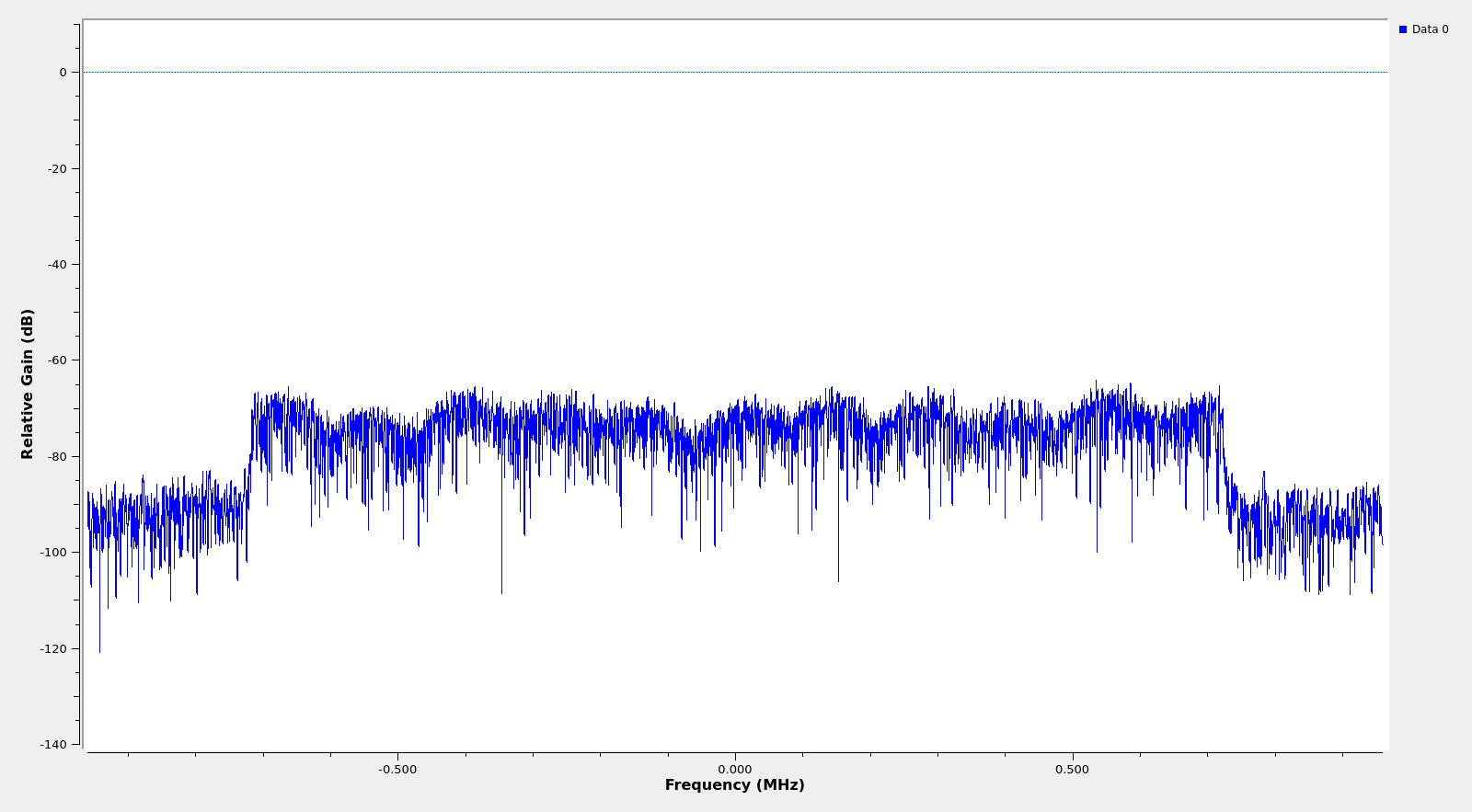
In doing this, I wanted to avoid the textbook approach of “assume that the signal is synchronized”. I wanted all kinds of synchronization to be a part of the challenge. I didn’t want to make things unnecessarily difficult, so I took care that the SNR was high enough, that the multipath was not too crazy, etc. This is how the spectrum looked like. I made sure to leave at least around 20 dB SNR in every subcarrier.
For the SigMF metadata, I decided to add some subtle references to LTE, but I didn’t intend to confuse anyone in thinking that this was really LTE. The sample rate for the file was 1.92 Msps, which is the sample rate used for an LTE carrier with 1.4 MHz bandwidth, and the centre frequency was 1810.75 MHz, which is somewhere in the middle of the downlink B3 band, which is a very popular LTE band.
This challenge was solved successfully by orangerf. Congratulations! They told me that they had worked previously on reverse-engineering some other OFDM signals. I don’t have a full solution to show here, but at least I’ll give some indications.
The frame structure was easy to see in the waterfall, for instance using inspectrum. The pilot symbols were easily seen by their pattern (in hindsight it was very good that I repeated a relatively short sequence to form the pilots), and the length of the symbols could be found by the keying clicks caused by symbol changes. Here I have used cursors to mark the 8 symbols in a frame by hand. Note that I have obtained a symbol duration of 600 us, which is exactly right.
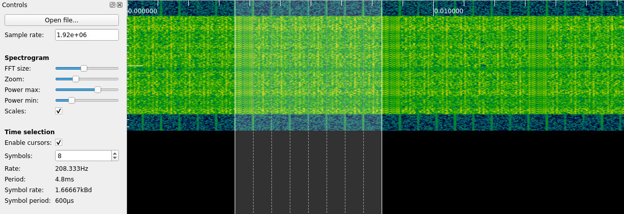
The useful symbol length (and hence the carrier separation) could be found by using the autocorrelation of the signal. Due to the cyclic prefix, there will be a strong autocorrelation peak at the lag given by the symbol length.
An alternative way of finding the symbol length was deduction/guesswork. The symbol duration we have found is 1152 samples. This is somewhat larger than 1024 samples (in fact it’s 1024 samples times 9/8). If I am giving the IQ file in the same sample rate that this OFDM modem supposedly uses, then 1024 samples looks like a very reasonable FFT size, and hence the useful symbol duration should be that (recall that the FFT size of an OFDM modem is equal to the useful symbol duration in samples, and that for efficiency, it should be a power of 2 or a product of powers of small primes).
Once we know these parameters, we can obtain a coarse time alignment from the waterfall and attempt to demodulate a symbol. Since I put a carrier offset frequency of several subcarriers, we are not done yet. The subcarrier separation is 1875 Hz, and the carrier frequency offset (still unknown to us) is 3728 Hz. At this point we only need to determine the carrier frequency offset modulo the subcarrier separation, so that the subcarriers of the signal are correctly aligned to FFT bins. Once we achieve that, we can count how many FFT bins are occupied by subcarriers, note that our frequency offset is off by a few subcarriers, and fix it if we want.
The subcarrier frequency offset can be found by hand (after all, the only thing we need is that most of each FFT bin is occupied by a subcarrier, instead of having half of the bin occupied by one subcarrier and the other half by the adjacent subcarrier). Alternatively we can also use the variant of Schmidl & Cox that I mentioned in my post about the LTE uplink. The phase of the correlation peaks that we obtain with this method gives an estimate of the carrier frequency offset.
After we do this, we have coarse estimates for the symbol time offset and the carrier frequency offset. We can demodulate a pilot symbol and see that the constellation is QPSK. If we look closely at this pilot symbol, we will see that it is formed by 48 repetitions of the same 16-symbol sequence. We were given a 32-bit syncword in the challenge description, so now we connect the dots and realize how the pilot symbols work.
At this point we can estimate the channel using this pilot symbol. Since the channel doesn’t change with time (which is apparent in the waterfall from inspectrum), this estimate is valid for all the IQ file. Now we can attempt to demodulate and equalize all the symbols in the IQ file. When we do this we will be able to refine our carrier frequency offset and we will also note that there is a sample frequency offset and correct for it. This can be done as in my LTE posts (for instance, on the one about the uplink).
Once we have demodulated the data symbols, I guess that it’s not too hard to realize that there is ASCII text, and putting all the demodulated data together, we can just grep for the flag.
Never the same color
This was a track of challenges made by Clayton Smith (argilo). I managed to solve all the challenges in this track, and since Clayton liked the way in which I solved it, he invited me to share my solution in the CTF walkthroughs that we did on Friday. Hence, I’m also including my solution to these challenges here.
When I opened the IQ file with Inspectrum, I immediately realized that this was a video signal. Then I connected dots and said “oh, Never The Same Color”, remembering the saying about NTSC. There was also a reference to the back porch in the challenge description:
While sitting on my back porch, I noticed a strange signal and made a SigMF recording. Can you make any sense of it?
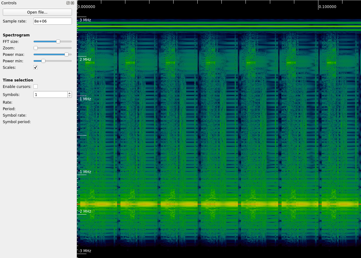
I didn’t know that much about NTSC, and learned a lot with these challenges, so this part of the Wikipedia page on NTSC helped me quickly get the information I wanted. I first wanted to look at the audio subcarrier, since that would be the easiest to handle. According to Wikipedia it is FM modulated and in the upper part of the spectrum. We can see it at ~2.75 MHz in the waterfall above.
Thinking that there might be additional signals hidden in the audio subcarrier (this had already happened in the Signal identification challenge, where a broadcast FM signal had flags in the mono, stereo and RDS channels), I made a simple GNU Radio flowgraph to FM-demodulate the audio subcarrier and drop it to a file that I could use with Gqrx. Since Gqrx only handles IQ files, but the FM demodulator output is real, I made a complex signal by putting zeros in the imaginary part. In this way we get a symmetric spectrum, but all the information is there.
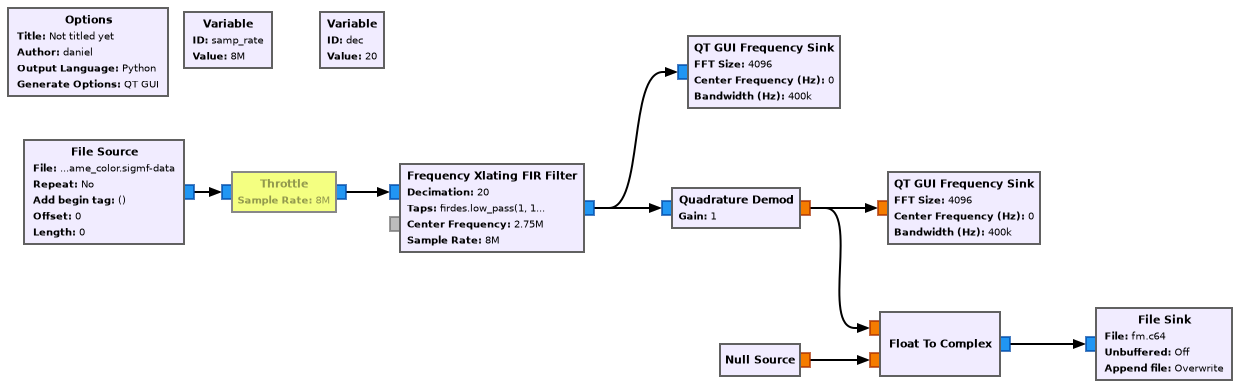
I found a bunch of flags quickly by demodulating this file in Gqrx in USB and FM modes. Most of these flags were on additional audio subcarriers that are specified by the NTSC standard (second audio program and so on), and the flags said so, but I went so fast through this that I didn’t pay much attention.
Once I was convinced that most likely there were no more flags in the audio, and missing 3 flags out of a total of 7, I set to work with the video. Rather than using SigDigger, SDRAngel, or some other ready-made software to decode the video, I thought of doing my own crappy decoder in Python. The reason was that I’ve sometimes heard that these applications can be a bit finicky regarding synchronization of the video signal, and that I thought that if there was something hidden in the video signal, my chances of finding it were better if I had to handle the signal by hand. This is the part of my solution which is interesting, because other participants used one of these applications (sometimes finding problems) or an actual TV to decode the video.
What I did first is to demodulate the luma component by using a Frequency Xlating FIR Filter centred at -1.75 MHz (which is where the luma carrier was) with a lowpass filter having a cutoff of 3 MHz, followed by a Complex to Mag block. The filter was used to get rid of the chroma and audio subcarriers. I didn’t give any thoughts to how the fact that the luma is vestigial sideband should affect the demodulation, but this approach worked fine. On second thoughts, for best results it is necessary to handle the vestigial sideband by doing something clever. Also, my idea to centre the filter at the luma subcarrier was plain silly, since for AM demodulation it doesn’t matter that the signal at the output of the filter is centred. It would have been best to center the filter in the middle of the portion of the signal that we want to extract, which is asymmetric about the luma carrier.
The GNU Radio flowgraph for this is shown here. At this point I didn’t have yet the Polyphase Arbitrary Resampler. I’ll come back to it later.
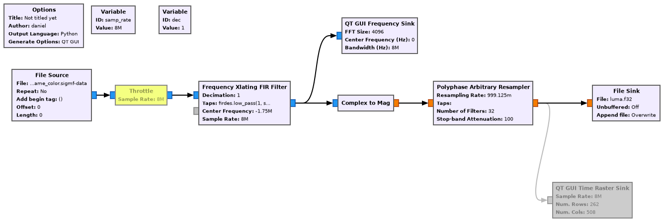
I thought of maybe using GNU Radio to display the video, but the SDL Video Sink block was missing on my machine and the Time Raster Sink is not very good for this. Instead, I used a Jupyter notebook to arrange the time domain luma signal into images. The approach was similar to the one I have described for the SETI challenge, except that here the line length is known. A quick Google search shows that the NTSC line frequency is 15734.25 Hz. This means that at 8 Msps there are around 508.44495 samples per line.
We can round this number to 508 samples and use this line length to plot the first field of the video. As shown below, the image is very slanted. Still there is a QR code which we can de-slant with GIMP and read. However, this is a rickroll.
I had the idea to look at the rest of the video, since the image could change at any point. But to do this, it was a good idea to get rid of the slant first. Large slants like this happen specially when the line length in samples is short. We need to round it to the nearest integer, and the relative error made by this rounding is large. A simple trick is to interpolate the data to make the line length longer, so that the relative error caused by rounding decreases. A better trick, specially when we know the exact line length, is to use an arbitrary resampler with a resampling ratio close to one to make the line length be an integer number of samples.
That is the purpose of the Polyphase Arbitrary Resampler block in the flowgraph above. It makes the line length equal to exactly 508 samples, rather than 508.44. Note that this approach only works if there is no sample rate offset. If we were dealing with a signal that involves real hardware, there will typically be a sample rate offset of a few ppm, but Clayton has been nice and has included no sample rate offset in this file.
The Polyphase Arbitrary Resampler approach works even in the presence of a sample rate offset, but we need to estimate the offset (by measuring the slant on the images) to refine the resampling ratio. With real hardware the sample rate offset will change with time, so this approach breaks down. A more complicated demodulator that uses the horizontal blanking interval to perform synchronization is need. However, for a short recording this simple approach might be okay, even with real hardware.
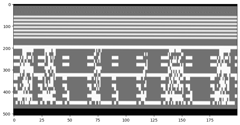
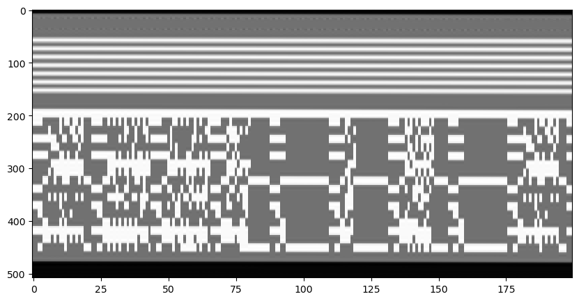
Once we do the resampling, we get perfect images with no slant. As part of these images we can see all the parts of the data which would normally be outside the screen are, which are called blanking intervals. The figures below shows the first field (even lines), the second field (odd lines), and the deinterlaced framed.

Once I was happy with my code, I wrote a loop that wrote each frame to a PNG file with Pillow. Then, I looked through these images with feh.
While quickly browsing the frames, I noticed that there were some horizontal lines white lines on the top of the image that changed every frame (we can see them in the figures above and below). Besides this, the image was static. However, when I arrived at frame 112, I noticed that the QR code changed.


The QR code changed back to the usual on frame 113. The QR code from frame 112 contained a flag. This special QR code appeared in other frames further down the IQ file, but each time only in a single frame, to make it difficult to see or catch to those playing the video in real time.
Missing two flags now, I decided to investigate the white lines above the image. I thought that maybe if joined these lines in all the frames together, I would get some kind of image, so I wrote some Python code to do that, and got the following. Here each frame corresponds to two columns of the image, and only the first 400 frames are shown.
We note that there is some kind of even/odd pattern in the columns, so maybe we need to group even and odd fields together. We get the following.
Still it was not clear to me what this is. It doesn’t seem like a crazy kind of barcode. Perhaps digital data of some sort, without scrambling, of course. Then I thought of teletext (I’m old enough to have used teletext as a child, but it was the PAL one). Up to this moment I was thinking of some custom way of embedding the flag just for this challenge, but maybe a standard method covered by NTSC was used. The teletext data must surely be sent somewhere in the video signal, and a quick search showed me that it occupies a portion of the vertical blanking interval, just like this data.
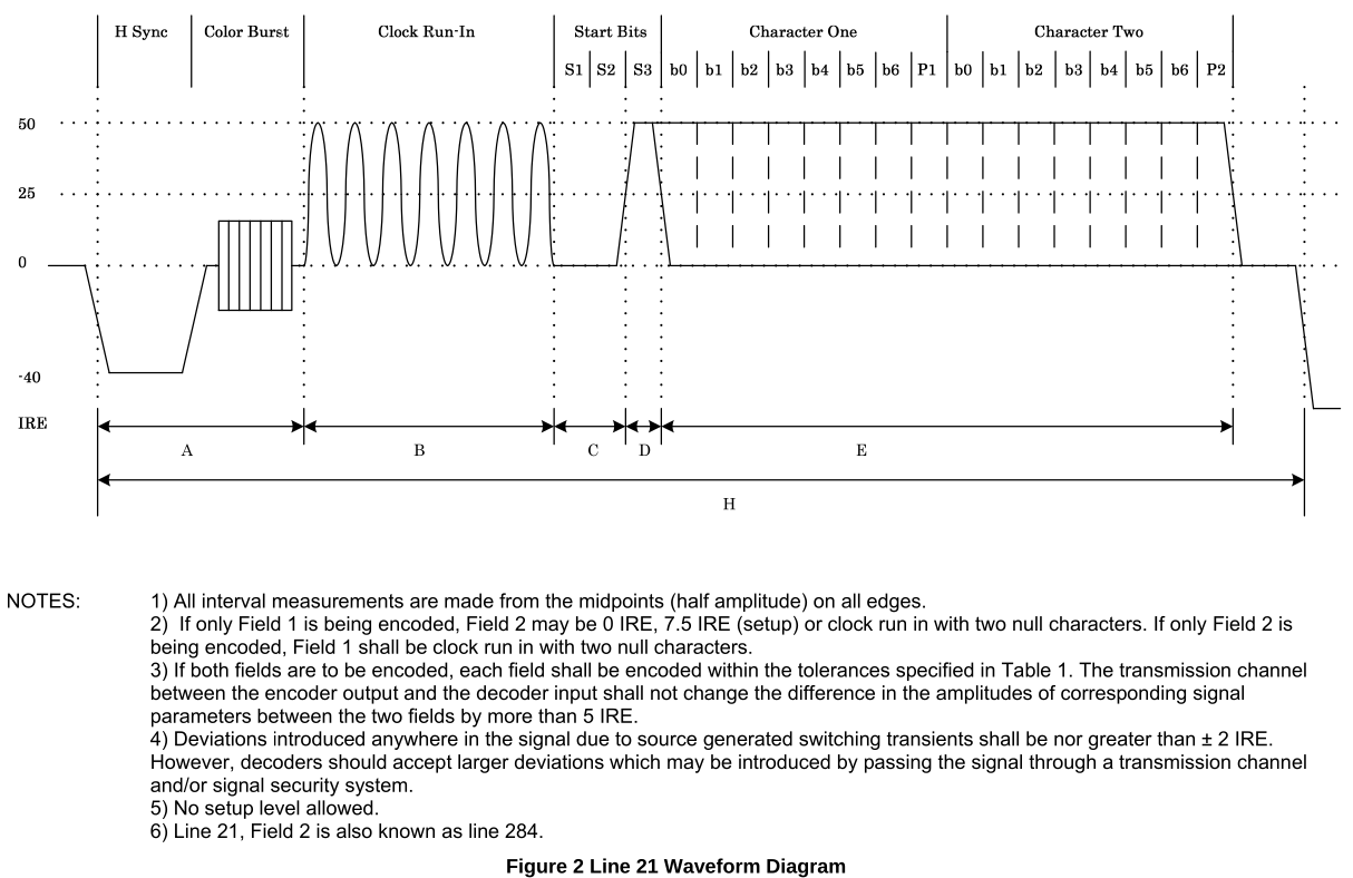
However, all of what I read pointed to a much higher data rate than what I was seeing here. Then I came accross line 21 closed captions (also called EIA-608 or CEA-608). This was a way of sending closed captions digitally in the line 21 of the vertical blanking interval of NTSC. The data rate looked very much like what I was seeing.
I got my hands on the standards document (you need to “buy” it to download it, but it’s actually free), and saw the following figure. It matched perfectly the data in the CTF file.
I took the the first line of data and recovered the clock by hand, as shown here. Note that the clock run-in goes high and low in each bit duration, unlike the usual digital signals where we have a 101010 kind of signal. The same clock recovery was valid for all the fields.
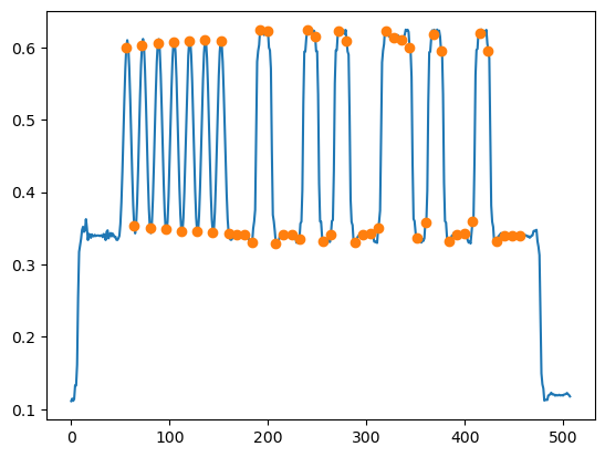
Then I sliced the bits, checked the parity just as a sanity check, and printed the data corresponding to the even fields, taking advantage of the fact that the character set used by EIA-608 is almost like ASCII. There was the rickroll URL again, but also the flag
Part 6: flag[21-is-the-magic-number]
I then did the same with the data in the odd fields. I could see something, but the characters were garbled. This is supposed to say “Part 7: flag[whatever]”:
Cneg 7: synt[pp3-sbe-gur-jva]
The numbers and symbols were readable, but the letters were not. I had seen that EIA-608 had character sets for Cyrillic, Chinese, etc., so I spent some time searching if there was a character set for the latin alphabet where the numbers and symbols were like ASCII but the letters were permuted. I even considered EBCDIC. At some point, rot13 dawned on me and I got the flag.
Closing
The CTF was really fun and enjoyable, and there were other very remarkable challenges that I haven’t covered here, such as the Dune track by muad’dib and the “SDRdle” by argilo (a wordle game played with APRS messages and spectrum painting). Thanks to all the people who submitted challenges and to all the participants.
3 comments