Since a couple months ago, the QO-100 NB transponder has now two digital beacons being transmitted continuously: the “traditional” 400 baud BPSK beacon, and the new 2.4 kbaud 8APSK multimedia beacon. This transponder is an amateur radio bent-pipe linear transponder on board the Es’hail 2 GEO satellite. It has an uplink at 2400.25 MHz, a downlink at 10489.75 MHz, and 500 kHz bandwidth. The two beacons are transmitted from the AMSAT-DL groundstation in Bochum, Germany, with a nominal frequency separation of 245 kHz.
In some posts in the last few years (see this, for instance), I have been measuring the frequency of the BPSK beacon as received by my grounstation in Madrid, Spain. In these frequency measurements we can see the daily Doppler curve of the satellite, which is not completely stationary with respect to the surface of Earth. However, we can also see the frequency variations of the local oscillator of the transponder (including some weird effects called “the wiggles“). For this reason, the frequency of the BPSK beacon is not an ideal measurement for orbit determination, since it is contaminated by the onboard local oscillator.
If we measure the frequency (or phase) of the 8APSK and BPSK beacons and subtract the two measurements, the effects caused by the transponder local oscillator cancel out. The two beacons have slightly different Doppler, because they are not at the same frequency. The quantity that remains after the subtraction is only affected by the movement of the satellite.
Bochum and my station use both references locked to GPS. Therefore, the phase difference of the two beacons gives the group delay from Bochum through the transponder to my station. This indicates the propagation time of the signal, which is often known as three-way range. The three-way range is roughly the sum of distances between the satellite and each groundstation (roughly, but not exactly, due to the light-time delay). It is a quantity that is directly applicable in orbit determination.
In this post I present my first results measuring the phase difference of the beacons and the three-way range.
Measurement set up
I have already described my QO-100 groundstation in other posts. For this experiment, it is relevant to say that a Vectron MD-011 GPSDO is used to generate a 10 MHz frequency reference, from which 27 MHz is obtained with a DF9NP PLL. The 27 MHz signal is used as reference for an Avenger PLL321S-2 Ku-band LNB, and for a LimeSDR mini. The LimeSDR mini streams 600 ksps IQ data into a BeagleBone Black, which uses the Linrad network protocol to send the data over Ethernet to a PC running GNU Radio.
All the processing of the two beacons is done in GNU Radio. The phase of the beacons is measured by locking a Costas loop to each beacon and reading the internal phase variable of the loop. For the BPSK beacon we use the usual Costas Loop block. For the 8APSK beacon we use the 8APSK Costas Loop that I presented in this post.
Each of the beacons is downsampled to 6 ksps before the Costas loop. The Costas loops run before symbol synchronization, because we need a known and fixed sample rate to take the phase measurements (the symbol synchronization performs variable resampling to align itself to the sample clock). The drawback of this method, in comparison with the more common approach of running the Costas loop after symbol synchronization, is that the Costas loop sees less SNR, so it has higher squaring losses. After the Costas loop we perform symbol synchronization, but this is only used to plot the constellation to check that the signal quality is good.
Initially I intended to process each of the two beacons independently. However, I found that the 8APSK Costas loop had cycle slips every now and then. This is not surprising, because the 8APSK constellation has 7 points around the unit circle, which increases the chances of cycles slips. Unable to fix this problem by playing with the Costas loop bandwidth, I decided to solve it in another way. The internal phase of the Costas loop of the BPSK beacon is subtracted from the phase of the 8APSK beacon before the 8APSK Costas loop. This “steering” removes most of the phase/frequency changes that the 8APSK Costas loop sees. Therefore, we can run the 8APSK Costas loop with a very small loop bandwidth. This prevents cycle slips.
The GNU Radio flowgraph is designed so that there are no accumulating phase errors due to floating point arithmetic. In particular, the local oscillators for downconversion are generated as periodic sequences using the Vector Source (see this post for more details about this and other relevant tricks when doing phase/frequency/timing metrology). The only local oscillator generated with a Signal Source (which has arithmetic problems) is the one used to cancel the small frequency offset (around -100 Hz) of both beacons, which is mainly due to the frequency error of the transponder local oscillator. This local oscillator is mixed with both of the beacons, so its effects cancel out in the phase difference.
The flowgraph writes phase measurements to a file at a rate of 200 sps. These consist of:
- The internal phase of the 8APSK Costas loop, which is actually the phase difference between the 8APSK and BPSK signals due to the steering described above.
- The internal phase of the BPSK Costas loop.
If needed, the phase of the 8APSK beacon could be computed by summing these two measurements.
Another aspect which is important for running the flowgraph reliably is handling dropped samples. Any dropped sample that is not accounted for will produce a jump in the phase difference measurement. The IQ samples are sent through the network in UDP packets using the Linrad network protocol. Occasionally, some of these UDP packets will be lost. Since the Linrad network packets have a packet number counter, lost UDP packets can be accounted for by inserting the necessary number of zeros in the IQ stream. I have added a new C++ block to gr-linrad that performs this task.
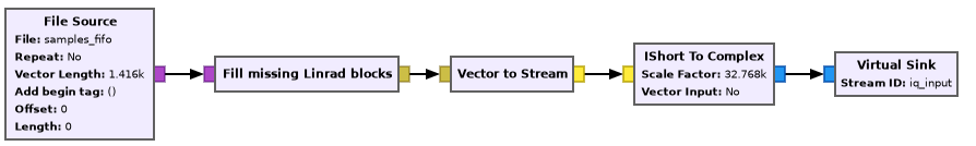
The figure below shows the input section of the GNU Radio flowgraph. A File Source reads from a FIFO the data coming by UDP. I have used this together with
socat -u udp-recv:50100 pipe:samples_fifo
because I was having some issues with GNU Radio’s UDP Source block. The data then goes to “Fill missing Linrad blocks”, which regenerates dropped UDP packets by inserting zeros in the data stream. Finally, we convert the samples to complex format.
To process the 8APSK beacon, the IQ data is shifted using an exact -245 kHz local oscillator and decimated to 6 ksps in two steps. Then we multiply with a local oscillator freq_corr, which is also used with the BPSK beacon and accounts for the frequency error of both beacons, mainly caused by the error of the transponder local oscillator (around -100 Hz). There is also another local oscillator offset_corr. This is an exact -1.6 Hz oscillator. It is used because I have observed that the frequency separation of both beacons is approximately 1.6 Hz larger than the nominal 245 kHz (more on this later).
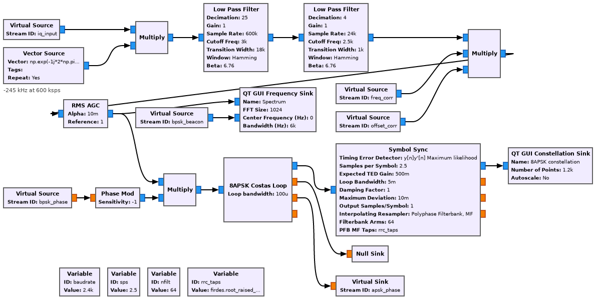
After multiplication by these local oscillators, we apply an AGC. A Phase Mod block uses as input the phase of the BPSK Costas loop to generate a complex exponential of the opposite phase. This is multiplied with the 8APSK signal to steer it. After this, we can run the 8APSK Costas Loop with a very small bandwidth, and then the Symbol Sync.
The processing of the BPSK beacon is similar. The main difference is that a regular Costas Loop is used instead of the specific one for 8APSK, and that no steering is done.

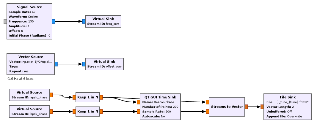
The remaining part of the flowgraph contains the freq_corr local oscillator, which is generated with a Signal Source, as mentioned above, and the offset_corr local oscillator, which is generated as a precision -1.6 Hz local oscillator. This part also contains the output section, in which the phase measurements of the Costas loops are downsampled to 200 sps and written to a file.
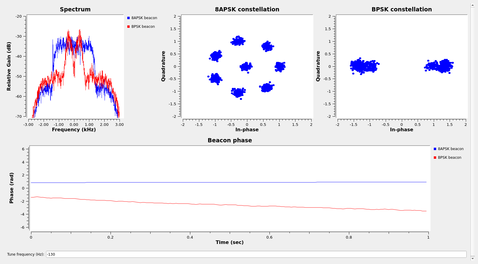
The figure below shows the GUI of the flowgraph. This includes the spectrum of both beacons and their constellation plots. There is also a time domain plot of the phase outputs. By counting how many phase wraps happen in one second, it is possible to estimate the frequency of the BPSK beacon. The frequency of the phase difference output (8APSK Costas loop output) is quite low, so it takes many seconds for its phase to wrap. Still, it is possible to see the value of the phase moving slowly.
Measurement post-processing
The phase measurements are post-processed in a Jupyter notebook. The phase output of the 8APSK Costas loop is unwrapped to obtain the phase difference between the 8APSK and BPSK beacons. The result cannot be interpreted directly, because of the following two reasons, which will be explained in more detail in the measurement limitations section below:
- The frequency separation of the beacons is not exactly the nominal 245 kHz. The error in frequency separation, which is not know exactly, produces a linear slope with respect to time in the phase difference measurement.
- Phase measurements are ambiguous modulo one cycle. Additionally, we do not know the phase difference at the transmitter in Bochum at any particular UTC timestamp, and we don’t have accurate UTC timestamps in our data. These effects cause an unknown offset (which can be any real number) in the phase difference measurement.
Since the consequence of these two points is the addition of a linear polynomial to the phase difference data, we use the detrend function from SciPy to fit and remove a polynomial of degree one from our phase difference measurements. This has the drawback that we will not obtain the correct three-way range, but rather a detrended version of it. Still, this allows us to see the relative changes of the three-way range over time. The main problem is that our three-way range is most likely contaminated with the wrong slope with respect to time. To fix this problem, it is necessary to determine the frequency separation between the beacons exactly. I will attempt to do this in the future.
The Doppler of the BPSK beacon is computed from the phase measurements of the BPSK Costas loop. The Doppler frequency can then be used for comparison. To obtain the Doppler, the phase measurements are unwrapped, and then phase measurements in suitable time intervals according to the desired integration time are differenced. I am using an integration time of 10 seconds, which already gives good results.
It is worthy to mention that a direct comparison between the Doppler of the beacon and the three-way range is not possible. Intuitively, the time derivative of the three-way range, which is called three-way range-rate, speaks of how the distance between the satellite and groundstations changes. The Doppler also speaks of the same thing. However, the problem is that with a bent-pipe linear transponder, the Doppler weights differently the distances on the uplink leg and on the downlink leg.
To show this, let us assume for simplicity that the references of the groundstations and satellite transponder are perfectly synchronized to the same timescale. We denote by \(t_{RX}\) the reception time at the receiving groundstation, by \(t_{S}(t_{RX})\) the time at which the signals received at \(t_{RX}\) were retransmitted by the satellite transponder, and the by \(t_{TX}(t_{RX})\) the time at which these signals were originally transmitted by the transmitting groundstation. We denote by \(f_1\) and \(f_2\) the uplink frequencies of the two signals we are using, and by \(f_{LO}\) the transponder local oscillator frequency.
The phase \(\varphi_j(t_{RX})\) measured in the receiving groundstation for each of the two signals is\[\varphi_j(t_{RX}) = f_j t_{TX}(t_{RX}) + f_{LO} t_S(t_{RX}).\]Therefore,\[(\varphi_1 – \varphi_2)(t_{RX}) = (f_1 – f_2)t_{TX}(t_{RX}),\]so we get\[\frac{d(\varphi_1-\varphi_2)(t_{RX})}{d t_{RX}} = (f_1-f_2) \frac{d t_{TX}(t_{RX})}{d t_{RX}}.\]The term \(d t_{TX}(t_{RX})/d t_{RX}\) that shows up here is essentially the three-way range-rate (but with the opposite sign).
On the other hand,\[\frac{d\varphi_j(t_{RX})}{d t_{RX}} = f_j \frac{d t_{TX}(t_{RX})}{d t_{RX}} + f_{LO} \frac{d t_S(t_{RX})}{d t_{RX}}.\]The term \(d t_S(t_{RX})/d t_{RX}\) which didn’t appear above corresponds to the range-rate of the downlink leg only. Therefore we see that the Doppler on each of the two signals separately consists of the three-way range-rate weighted with \(f_j\), plus the downlink-leg-only range-rate weighted with \(f_{LO}\).
This behaviour is characteristic of a bent-pipe linear transponder. In a turnaround transponder such as those used in deep space navigation, this doesn’t happen. Such a turnaround transponder receives a phase modulated signal on the uplink, multiplies by some constant (called the transponder turnaround ratio) the frequency of the uplink carrier to generate the downlink carrier, demodulates the phase modulated information on the uplink, and remodulates it on the downlink carrier.
For the turnaround transponder, the formula for the received phase is\[\varphi_j(t_{RX}) = \alpha_j f_j t_{TX}(t_{RX}).\]Here \(\alpha_j\) is the transponder turnaround ratio if the signal under consideration is the uplink carrier (in which case \(f_j\) is the uplink carrier frequency), and \(\alpha_j = 1\) if the signal under consideration is modulated on the uplink carrier using a subcarrier (in which case \(f_j\) is the subcarrier frequency). We see that in the turnaround transponder, the downlink-only term \(t_S(t_{RX})\) doesn’t ever show up, so some of the treatment is simplified.
To compute three-way range-rate, we difference the range measurements in time intervals according to the integration time. An integration time of 100 seconds works well to reduce the noise. The convenient thing of using range-rate is that the unknown polynomial of degree one that we had in our range measurements now turns into a constant. Therefore, the range-rate measurements are only wrong by a constant offset.
Measurement limitations
As remarked above, the phase difference measurements cannot be used directly, as they are contaminated with two effects. The first of these is caused by the fact that we don’t know the exact frequency separation of the two beacons. This is caused by two effects compounded:
- At the transmitter, the frequency separation is not exactly 245 kHz. Often, when working with SDR, it is not easy to achieve exactly the frequencies we want. There are both software causes and hardware causes for this. In software, depending on how the calculations are done, quantization errors will generate a slightly different frequency from the desired one. In hardware, fractional-N synthesis errors in the PLLs cause the frequencies for the local oscillators and data converter clocks to be slightly off. On this note, AMSAT-DL mentions that the BPSK and 8APSK beacons are generated from two different ADALM Plutos locked to the same reference.
- At the receiver, due to fractional-N synthesis errors, the sample rate of the ADC of the LimeSDR is not the nominal 600 ksps. These errors are investigated in a section below.
Ideally, exact values for all of these effects can be found by examining how the system is implemented, looking at the datasheets of the PLLs and RFICs, etc. Note that the frequency errors of the receiver need to used to correct the phase difference measurements. However, the frequency errors of the transmitter need to be taken into account both to correct the phase difference measurements and also to convert the measurements to units of distance or time, since as shown above, the measurements are proportional to the difference \(f_1 – f_2\) of actual uplink frequencies. If these effects are handled correctly, then the unknown phase versus time slope in the three-way range measurements will disappear.
The second effect that contaminates the measurements is a constant offset. In principle, every time that we work with phases we have this kind of offset, since phase measurements are only valid modulo one cycle. Therefore, there is always an unknown offset that consists of an integer number of cycles. Under certain circumstances, this integer ambiguity can be solved exactly (since it is an integer) using other known data.
In our case we are dealing with Costas loops, which have ambiguities that are of a fraction of a phase cycle. The BPSK Costas loop has an ambiguity of 1/2 cycle, and the 8APSK Costas loop has an ambiguity of 1/7 of a cycle. Potentially these ambiguities could be solved (to obtain an ambiguity of one cycle) by looking at the symbol stream. For instance, the syncwords of the 8APSK beacon give us the correct phase modulo one cycle. Nevertheless, we are not doing this for simplicity, so when computing the phase difference we have an ambiguity of 1/14 of a cycle rather than one cycle.
Besides these phase ambiguities, here we have a larger problem, which is that we don’t have any synchronization between the timescale (say, UTC) and our phase measurements. At the transmitter, we don’t know the phase difference between the two signals at any particular timestamp. Presumably we could know how the phase difference evolves with time, if we find the exact frequency separation. But still this leaves us with an unknown constant offset which can be any real number. This problem is difficult to fix, specially because the signals are transmitted from two different SDRs.
Similarly, in the receiver we don’t have any precise relation between the IQ samples that we get from the LimeSDR and the timescale. This would be relatively easy to fix by timestamping the IQ samples to a 1PPS signal.
The consequence of this is that there is a constant unknown offset in our three-way range measurements that is quite difficult to solve. Nevertheless, if the measurements are used for orbit determination, the offset (or actually, an estimate for it) could be found as an additional unknown in the least squares fit process.
Another limiting factor is the time synchronization of the transmitter and receiver. These use GPSDOs as references. Therefore, the two references won’t drift with respect to each other by much over long time periods. Still, the instantaneous time difference between them will usually be a few ns (perhaps 10 ns), so the measurements will be contaminated with this difference. This error can be reduced somewhat by averaging the measurements over time.
Experimental results
So far I have been running these measurements for around 49 hours, except for a power cut that caused some data loss. This power cut also caused the reset of the flowgraph, and hence of all the phase ambiguity information. Therefore, the data before and after the cut are detrended separately.
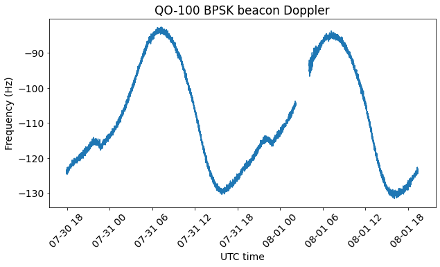
The first plot shows the Doppler of the BPSK beacon. There is a weird corner in the curve at around 21:00 UTC each day. As we will see with the phase difference data, this is caused by the local oscillator of the transponder rather than by the movement of the satellite.
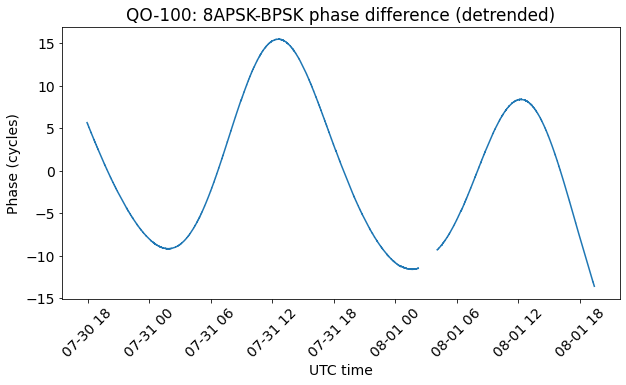
Here we see the phase difference measurements. The two curves have been detrended independently. They show the characteristic sinusoidal curve, but the detrend is introducing a wrong slope and offset in the data (the detrend would be more accurate if we considered many periods of the sinusoid).
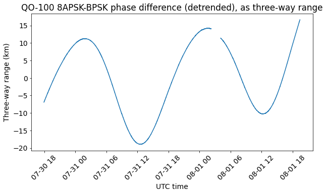
Passing from the phase difference to three-way range involves just a change in sign and units. We see that the three-way range varies by some 30 km every day.
The range-rate plot looks nicer because only the vertical offset of each of the two curves is wrong. We can clearly see that the offsets of the two curves don’t match together. There are some glitches in the range-rate, which appear as spikes in the plot. These are caused by jumps in the range measurement. The magnitude of the jumps is on the order of 60 m, so they are too small to be seen in the scale of the plot above. Nevertheless, these jumps are significant. They are investigated in the section below.
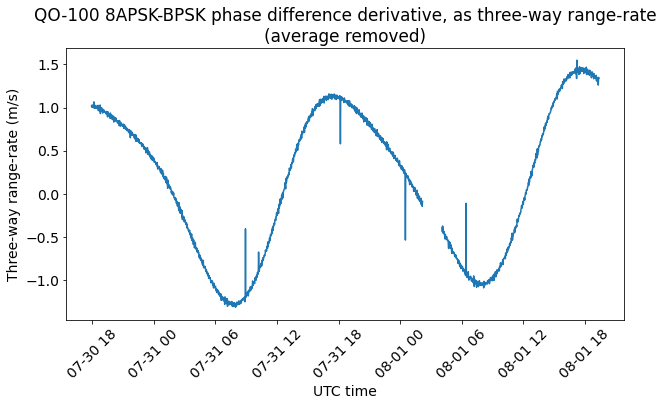
Another thing that we can see in the plot is that the range-rate doesn’t really follow a perfect sinusoid.
Glitches
The figure below shows a detail of the first glitch that was observed in the range-rate measurements. The detrended phase of the BPSK beacon is shown in blue, using the vertical scale on the left. The detrended phase difference is shown in orange, using the vertical scale on the right.
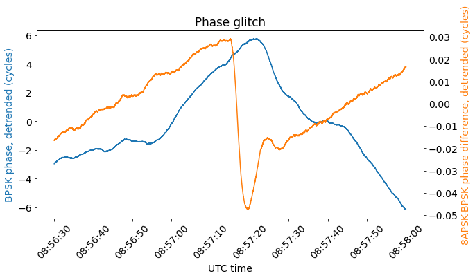
We see that at some point the phase difference jumps and establishes at a value which is approximately 0.05 cycles lower. The shape of the transient is given by the step response of the 8APSK Costas loop, which has a very narrow bandwidth.
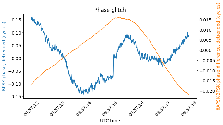
While not apparent in the plot above, the phase of the BPSK beacon also jumps at the same moment. This can be seen better in the plot below, which only shows 6 seconds around the event. In this case, the phase of the BPSK beacon jumps by 0.1 cycles or so.
The other glitches look similar. Their plots can be seen in the Jupyter notebook.
I am not sure of what is the cause of these glitches. Note that if in the signal that we receive, only the phase of the BPSK beacon jumped, then due to the steering, in general the 8APSK Costas loop would also see a jump and would need to move to lock again. We would observe this as a jump in the phase difference. However, the magnitude of that jump would need to match the rotation needed to move to the closest 8APSK constellation point once we rotate the constellation by the magnitude of the BPSK jump. I have checked that this relation doesn’t hold between the magnitudes of the BPSK and phase difference jumps that we observe. The conclusion is that there are phase jumps in both signals.
A possible explanation would be that my receiver is dropping IQ samples. We are taking into account the dropped UDP packets. However, samples could be lost between the LimeSDR mini and the BeagleBone Black. I will try to see if I can at least detect and log these events to check if they match the timestamps of the glitches.
Note that the phase jumps that we see in the BPSK beacon are on the order of 0.1 or 0.2 cycles. Since such beacon is at a frequency of around -50 Hz in the IQ baseband, this means that we are losing around 2 to 4 ms worth of samples (assuming that we don’t lose much more and so we see phase wrapping on the phase jump). At 600 ksps this is 1200 to 2400 samples, so it could happen that we’re sometimes losing one of the USB transfer buffers (I haven’t checked the size of these buffers, but maybe it is of this order of magnitude). This idea also seems to agree with the fact that all the BPSK phase jumps, except for the first one, jump down. This would happen if we lose samples with a signal of negative frequency.
Another idea to explain this is that the jumps are caused by the transmitter at Bochum. Perhaps it is the transmitter the one that is losing samples. However, I find this explanation less likely, because the two beacons are transmitted from independent SDRs.
Fractional-N synthesis errors for the receive groundstation
I have made some initial calculations of the fractional-N synthesis errors of my groundstation. These have not been verified yet, so they should be used carefully. Still, they show that the errors caused by my station are small (but significant for this application), so most of the ~1.6 Hz error in the frequency separation of the signals is due to the transmitter at Bochum.
The first component that needs to be examined is the DF9NP PLL, which converts an input of 10 MHz into a 27 MHz output. This PLL uses the ADF4001 PLL chip. Looking at its datasheet, the most straightforward way to set this PLL to convert 10 MHz into 27 MHz is to use \(N = 27\), \(R = 10\), since the formula for the output frequency is\[f_{OUT} = REF_{IN} \times N / R.\]I imagine this is how the PLL is programmed in my case. This would mean that the PLL is generating exactly 27 MHz and not introducing any frequency errors. I still need to verify this, for instance by hooking up the 10 MHz and 27 MHz signals to an oscilloscope and checking that their relative phases don’t drift by.
The next element we need to consider is the LimeSDR mini sampling clock. Note that the frequencies of the local oscillator of the LimeSDR and of the LNB don’t matter, because they affect both beacons equally, so their frequency errors cancel out in the phase difference.
In the LMS7200M RFIC of the LimeSDR mini, I use the 27 MHz reference and an output sample rate of 600 ksps. Looking at the LimeSuite code, the LMS7_Device::SetRate method will choose an oversampling factor of 32 for this relatively low sample rate, so the ADC will run at 19.2 Msps. Since the CGEN runs at 4 times the ADC clock, this means that the desired CGEN frequency is 76.8 MHz.
Now we can look at the LMS7002M::SetFrequencyCGEN method to see how the fractional-N synthesis parameters are calculated. The VCO divider is chosen as 32, since iHdiv is computed as 15. Therefore, the VCO should run at 2457.6 MHz. Dividing the VCO frequency by the reference frequency of 27 MHz we get a ratio of 91.02222. The integer part is 91 (although in the code gInt is the integer part minus 1), and the fractional part is rounded down to 23301/1048576 (the value 1048576, which is \(2^{20}\), is the fixed denominator of the fractional-N synthesis). The rounding error is exactly 31/(45·1048576).
We can compute the actual output sample rate that we get, in MHz, as\[27 \cdot \left(91 + \frac{23301}{2^{20}}\right)\cdot \frac{1}{32} \cdot \frac{1}{4\cdot 32}.\]Here 27 MHz is the reference frequency, the term in parenthesis corresponds to the fractional-N feedback divider, the term 1/32 corresponds to the VCO output divider, and the term 1/(4·32) corresponds to the CGEN division and oversampling. This gives a sample rate which is ~4.33 mHz lower than desired, which is a 7.2 ppb error. The exact sample rate error is \(-3\cdot5^5\cdot31/2^{26}\) Hz, or \(-31/2^{32}\) parts per one (relative to the 600 ksps nominal sample rate).
The knowledge of the sample rate error \(\varepsilon\) in parts per one can then be applied to correct our phase difference measurements. The local oscillators that we are generating in GNU Radio to correct for the frequency separation of the two beacons, which have a nominal frequency of \(f_1 – f_2\), are wrong by \(\varepsilon(f_1 – f_2)\). Therefore, we should add a correction term \(\varepsilon(f_1 – f_2)t\) to the phase difference observations.
Note that this sample rate error gives an error of \(c \varepsilon \approx 2.16\) m/s in the range-rate calculations. This error is of the same order of magnitude as the range-rate itself (whose sinusoidal curve has an amplitude of approximately 1 m/s). Therefore, it is important to correct this error to obtain accurate results.
Strictly speaking, the error in sample rate also makes our timestamps wrong by \(\varepsilon\) parts per one, since we are deriving the timestamps just from counting samples. However, this effect is very minor for our application. Over an observation of 7 days, the error accumulates to only 4 ms. Since the range and range-rate change rather slowly, we do not need to be very accurate with the timestamps.
I still need to validate that my understanding of the LimeSuite code is correct and that these are actually the values that are being programmed in the LMS7200M. This can be done by modifying the code to print out these values or by using LimeSuiteGUI to look at how the values have been set. I haven’t done it yet because to do it I need to stop the measurement software.
Update 2022-08-03: I have now validated that the PLL parameters of the LMS7200M given above are the correct. With the LMS7200M in the usual configuration, I have run LimeSuiteGUI and save the data (essentially the register values) to a file. Then I have modified the reference frequency in the file, since LimeSuiteGUI insists that it is 30.72 MHz rather than 27 MHz. The file can be found here. When this file is opened with LimeSuiteGUI, the PLL parameters are shown. Note that the values for the fractional synthesis match those given above (except that the integer part is shown as 90 rather than 91).
Data and code
The material used in this post can be found in this repository, including the GNU Radio flowgraph, Jupyter notebook, and recorded phase measurements. The phase measurements are stored using git-annex and can be downloaded as described in this README.
2 comments