On July 13, the Vega-C maiden flight delivered the LARES-2 passive laser reflector satellite and the following six cubesats to a 5900 km MEO orbit: AstroBio Cubesat, Greencube, ALPHA, Trisat-R, MTCube-2, and CELESTA. This is the first time that cubesats have been put in a MEO orbit (see slide 8 in this presentation). The six cubesats are very similar to those launched in LEO orbits, and use the 435 MHz amateur satellite band for their telemetry downlink (although ALPHA and Trisat-R have been declined IARU coordination, since IARU considers that these missions do not meet the definition of the amateur satellite service).
Communications from this MEO orbit are challenging for small satellites because the slant range compared to a 500 km LEO orbit is about 10 times larger at the closest point of the orbit and 4 times larger near the horizon, giving path losses which are 20 to 12 dB higher than in LEO.
I wanted to try to observe these satellites with my small station: a 7 element UHF yagi from Arrow antennas in a noisy urban location. The nice thing about this MEO orbit is that the passes last some 50 minutes, instead of the 10 to 12 minutes of a LEO pass. This means that I could set the antenna on a tripod and move it infrequently.
As part of the observation, I wanted to perform an absolute power calibration of my SDR (a USRP B205mini) in order to be able to measure the noise power at my location and also the power of the satellite signals power, if I was able to detect them.
Observation set up
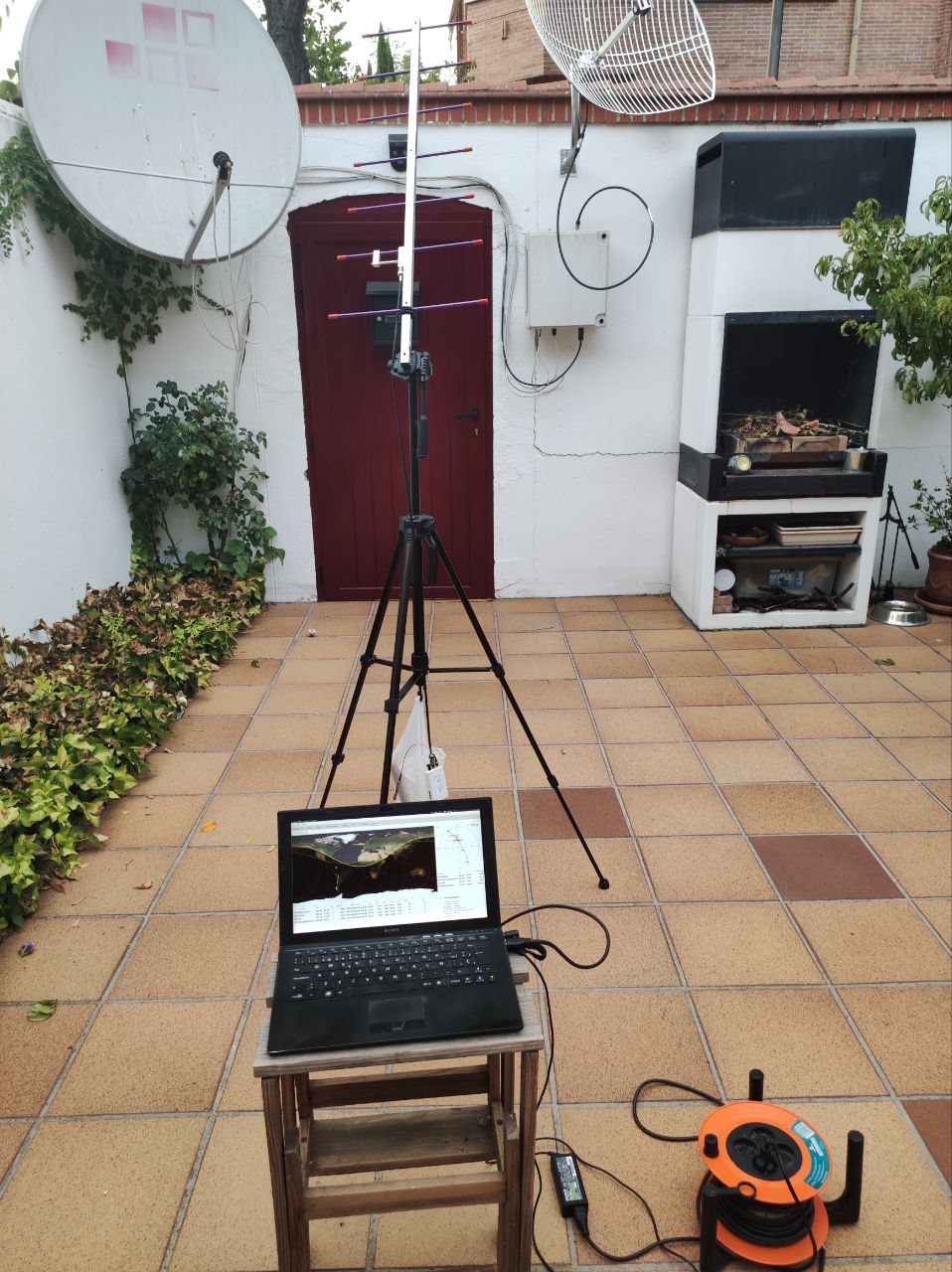
The hardware set up for the observation can be seen below. The yagi antenna is placed on a camera tripod and aimed by hand during the central part of a high elevation pass. A USRP B205mini is connected to the antenna directly through ~1.5 m of coaxial cable. The USRP is connected to a laptop running on mains power. (The antennas on the wall are my QO-100 groundstation, and not used in this observation.)
The observation is done with a GNU Radio flowgraph, shown below. The USRP is tuned to 436.52 MHz with a sample rate of 4 Msps. The downlink frequencies for four satellites are observed: CELESTA, MTCube-2, Greencube, and AstroBio CubeSat. I didn’t observe ALPHA and TRISAT-2 because I haven’t seen reports of other people being able to receive them. For AstroBio CubeSat, two frequencies are observed: 435.6 MHz (its nominal frequency), and 437.425 MHz since apparently the radio has been reset to the default factory frequency of 437.425 MHz.
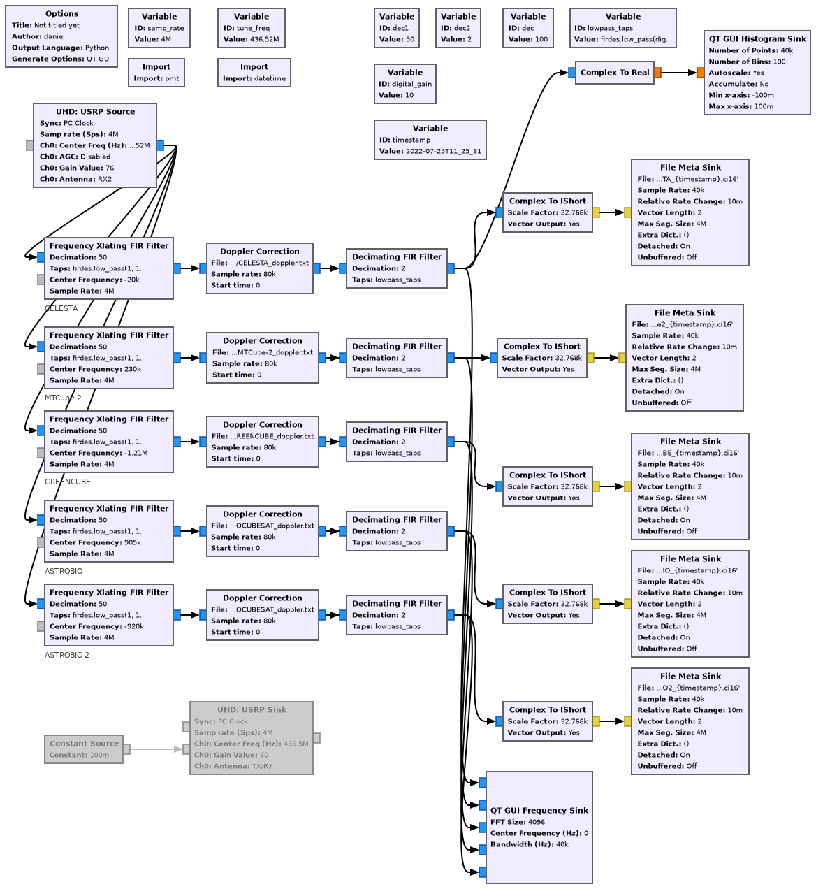
A Frequency Xlating FIR Filter block is used to obtain 80 kHz of spectrum around each of 5 frequencies to observe. Then the Doppler correction block is used to correct the downlink Doppler for each satellite. Another decimation reduces the sample rate to 40 ksps. The data is recorded in IQ format using 16-bit integers. The digital gain of the flowgraph is adjusted to make the most use of the 16-bit range while still leaving a headroom of around 20 dB.
The Doppler is computed using TLEs from Celestrak and Skyfield, and saved to text files as expected by the Doppler correction block (see this Jupyter notebook). The observation was done during the 2022-07-24 18:20 UTC pass over Europe. Three of the cubesats have very similar Doppler curves, since they are close together. AstroBio is lagging by some 15 minutes. The maximum elevation during this pass was 75 deg.
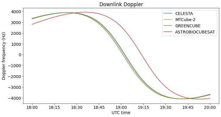
The observation was done between 18:47 and 19:24 UTC, when the satellites were at high elevation, as there are large buildings blocking the horizon at this location. The antenna was aimed by hand to the cluster of three satellites until approximately 19:19 UTC, when the cluster was descending through 40 deg elevation. At this moment, it was switched over to AstroBio.
Amplitude calibration
For the amplitude calibration of the SDR, I have followed the procedure that I described in this old post. Essentially, the calibration is traced to the fact that a GALI-39 MMIC LNA from Minicircuits has a rather stable noise figure of around 2.4 dB. A CW tone of unknown power is generated and connected to the input of the SDR directly. Then the same tone is connected through the GALI-39 to the SDR. In this latter measurement, the total noise figure is almost equal to the noise figure of the GALI-39, so we can measure the tone absolute power from its SNR. Once we know the power of the tone, we can establish the amplitude calibration using the measurement in which the tone was directly connected to the SDR.
This kind of amplitude calibration is accurate to perhaps 1 dB. The sources of error are the error in the noise figure of the GALI-39, losses in the connectors, changes in the parameters over time and with input/output impedance, nonlinearities of the SDR, etc.
To generate the CW tone, I used the USRP transmitter at a frequency of 436.5 MHz, matching the nominal frequency of CELESTA. The RX/TX port of the USRP was connected through a short SMA jumper cable to a 50 dB attenuator (actually 30 dB + 20 dB). Reception was always done through the RX2 port of the USRP. The TX gain of the USRP was set to 30 dB to give an adequate level at the USRP input. The UHD USRP Sink to generate the CW tone was included in the GNU Radio flowgraph but disabled during the observation of the cubesats. It was only enabled for calibration.
During the observation and the amplitude calibration, the RX gain of the USRP was set to its maximum value of 76 dB, in order to give the best noise figure possible (the SDR was far from saturation with this gain). Additionally, a digital gain of 10 was applied before quantization to 16-bits to save in the output files.
The gain calibration was done shortly after the observation of the cubesats, and in the same location, to have all the equipment running at the same temperature (the ambient temperature was around 35ºC due to the current heat wave in Europe). The RX/TX port was connected to RX2 through 50 dB attenuation and the TX output was enabled. Data was recorded for one minute using the same flowgraph, with the Doppler correction for CELESTA disabled. Then the GALI-39 amplifier was inserted between the 50 dB attenuator and the RX2 port, and data was recorded again for another minute.
The CW tone appears at DC in the IQ output for CELESTA. The figure below shows the IQ values and amplitude of the CW tone when it was connected directly to the USRP’s RX2 port. The 40 ksps IQ data has been averaged in segments of 100 ms to eliminate most of the noise. The average power of the CW tone can be measured directly from this plot.

The fact that the I and Q are changing in amplitude slowly is due to the fact that the CW tone is not exactly at 0 Hz. This is both due to uncorrected fractional-N synthesis errors in the USRP PLLs and perhaps also due to numerical errors in the NCO of the Frequency Xlating FIR Filter block in GNU Radio.
Note the oscillatory behaviour of the amplitude. I think this is caused by the USRP transmitter. I’ve observed it in other experiments, but I’m not certain about its cause. The frequency of these oscillations is a fraction of a Hz. Perhaps it’s the beat tone between the transmit local oscillator and the IQ data going to the DACs. The CW tone was generated at DC in GNU Radio, but the USRP uses the DUC NCO in its FPGA to correct the small frequency error of the AD9361 LO. Here I used an amplitude of only 0.1 for the CW tone in GNU Radio, so I guess that the beat tone effect would be larger than if an amplitude of 1.0 was used. In any case, these oscillations are not a problem for the amplitude calibration, since we measure average power.
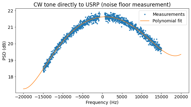
The next figure shows the spectrum. This is used to measure the noise floor power spectral density. Note that the noise floor is not quite flat.
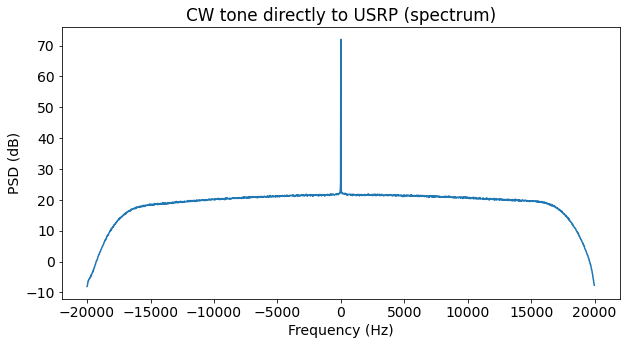
Since the noise floor is not flat, a polynomial of order 4 is fitted to the PSD measurements, ignoring the area close to DC, where the CW tone is present, and the edges of the passband. This polynomial then gives the noise PSD at DC, which is used for the calculation of the CW tone CN0. There is a 3 dB drop across the passband. I think this is caused by the filters in GNU Radio (specially because there are two filters). Next time I should be more careful with the filter design.
In the measurement through the GALI-39 unfortunately there was a problem that I only noticed when analysing the data afterwards. The signal level was too high and it saturated the 16-bit output of the IQ files. Below we can see the time domain output. We see that during most of the recording the I channel is saturated at 32767, but then the I channel decreases in amplitude, stops being saturated, and the Q channel enters saturation at -32768.
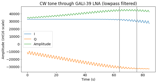
The Complex to IShort GNU Radio block saturates the output rather than wrapping around on overflow. This is both good and bad in this situation. It is good because we know for sure that it is barely saturating. If the output was wrap-around on overflow, we couldn’t know for sure how many wrap-arounds have happened. It is bad because whenever the output is saturated we lose all the information. If the output was wrap-around on overflow, then we could correct it using the knowledge of how many wrap-arounds have happened.
Luckily for us, there is a short segment where the I and Q channel are only saturating very little. It is marked with vertical gray lines in the plot above. In this segment, the amplitude measurement is correct. We use only this segment to measure the power of the CW tone. Since even in this segment there is some saturation, we are still underestimating the tone power, but only slightly.
Note that the saturation problem happens only digitally in GNU Radio. Since we are applying a digital gain of 10, the ADCs are at around -20 dBFs, and quite far from saturation. The correct way to perform this measurement would be to reduce the digital gain only for this case to prevent saturation.
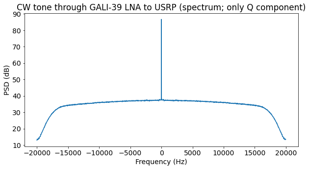
To measure the noise power, we use only the Q channel during the first part of the recording, where the Q channel is far from saturation. Then we can use the property that half of the noise power is in the I channel and half of the noise power is in the Q channel. Thus, we compute the spectrum of only the Q channel.
As before, we fit a polynomial of degree 4 to the noise floor in order to compute the PSD of the noise at DC.
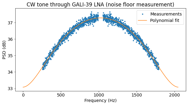
From these measurements we get that the CN0 of the tone is 63.3 dB·Hz when it is directly connected to the USRP and 65.6 dB·Hz when it is connected through the GALI-39. Assuming that the noise figure of the whole receiver including the GALI-39 is 2.4 dB, this gives a power of -104.0 dB for the CW tone. This, together with the amplitude of the tone when it is connected directly to the USRP gives us our amplitude calibration.
Additionally, from this calibration we obtain a noise figure measurement for the USRP of 5.6 dB and a gain for the GALI-39 of 21.0 dB. These are in the correct ballpark, so our calibration can’t be too far off. According to the GALI-39 measurements by Minicircuits, the gain of the amplifier should be around 22 to 23 dB (depending on the bias current and temperature). The USRP B210 (which is similar to the B205mini) was measured to have a noise figure of 4.4 dB at 437 MHz in the SDR Makerspace Evaluation of SDR Boards and Toolchains (see Table 2.24 in page 113).
I think that we have slightly underestimated the amplitude of the CW tone when it is connected through the GALI-39, due to the saturation problem. This would cause us to slightly overestimate the USRP noise figure and underestimate the GALI-39 gain, which seems consistent when comparing our results with other measurements. In any case, this amplitude calibration seems good enough for our purposes.
Note that the amplitude calibration has been done only at the frequency of CELESTA. Gain non-flatness in the USRP would be another source of error. This could be calibrated to some extent by using the data measured in the remaining channels while the GALI-39 was connected.
Preliminary analysis of the observation
The figure below shows a waterfall of the recording of CELESTA in Inspectrum. A weak packet from CELESTA can be seen in the middle of the waterfall. There are other much stronger and wider packets present, probably from a LEO satellite. The noise floor shows many spectral lines caused by RFI. The power and spectral shape of the RFI changes depending on where the antenna is pointed to. This is typical of RFI in urban locations.
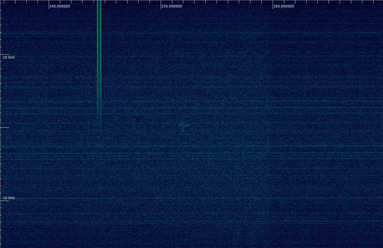
Packets from CELESTA can be seen every 40 seconds (though sometimes the packet is not visible), although they are quite weak. Sometimes only the spectral line in the “tail” of the packet is visible.
The results of this observation of CELESTA are much worse that this SatNOGS observation done from Hungary during the same pass. However, that observation was done with 4x 9 element yagis, and likely from a quieter location. Large fading in the signal from CELESTA can be seen in that observation.
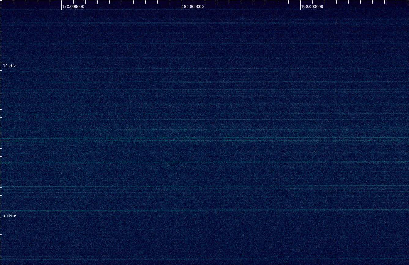
The signal of Greencube is very weak. Here it can be seen starting at 173 seconds, between 0 and 2 kHz. The satellite transmits a burst of packets almost continuously. There is a very slight enhancement in the power of the noise floor. Judging just from this waterfall, the enhancement could be anything. However, looking at some SatNOGS observations (6257949, 6256636, 6258354) done at the same time, we can match this with the bursts seen in the other observations (which have much better SNR). The burst starts at 18:50:34 UTC according to our recording. This is 316 seconds into observation 6257949, and 97 seconds into observation 6256636. Comparing closely the waterfalls of those two observations, there seems to be a time difference of 5.6 seconds between them. I don’t know how well they are synchronized to UTC.
Nothing has been detected in the channels of MTCube-2 and AstroBio Cubesat. There are no SatNOGS observations of those satellites showing signals during that pass either, so probably these two satellites weren’t transmitting.
Noise measurement
To measure the noise floor, we first compute a 2048 point waterfall of the 40 ksps IQ data using this GNU Radio flowgraph. Then, for each spectrum of the waterfall, we compute its mean and median. The motivation of studying the median is that the noise is far from being white Gaussian. It has many spectral lines that show up in the waterfall. These are outliers in the power spectral density. The median gives an estimator which is not so sensitive to outliers as the mean.
However, the median needs to be corrected for bias. Under the hypothesis that the noise is AWGN, each FFT bin in the PSD will be distributed as a constant times a chi-squared with 2 degrees of freedom. The mean of a chi-squared variable with \(k\) degrees of freedom is \(k\). Its median is approximately \(k (1-2/(9k))^3\). Therefore, we divide the median by \((1-1/9)^3\) to correct this bias.
The figure below shows the results of computing the average and median of the noise. Only the central 1/2 of the spectrum is used for this measurement to avoid the skirts at the band edges. The shape of the bandpass (which was determined in the amplitude calibration) is not taken into account for simplicity.
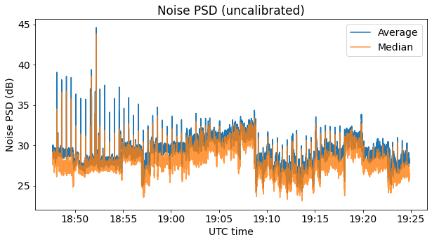
The sudden jumps in the PSD probably correspond to the moments in which I changed the antenna pointing manually. Besides this, the noise also seems to vary slowly when I didn’t move the antenna. Part of this could be attributed to gain changes (with temperature) in the USRP, but I think that part is actually the noise power changing even when the antenna doesn’t move.
Using the amplitude calibration determined above, the power can be converted to dBm. Since we have also determined the noise figure of the receiver, we can subtract it from the noise power in order to obtain only the power that is caused by antenna noise. This is shown below as noise power density in dBm·Hz and as noise temperature in K.
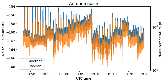
The noise temperature ranges between approximately 3000 and 10000 K. This is somewhat higher than what indicated in the ITU-R Radio noise models for city area man-made noise, but still in the ballpark. Compare this result with curve A in the figure below, which at 436 MHz gives somewhat above 3000 K of man-made noise.

It is not hard to imagine that the noise can be improved a lot by going to a quiet location. In this case the noise could be on the order of 300 K, dominated by ground thermal noise picked up by the antenna sidelobes. Using an LNA with a noise figure of 1 or 2 dB we could get a total receiver noise below 500 K. This would give an SNR improvement of 8 to 13 dB, allowing us to decode the signals from CELESTA, and probably also from Greencube.
CELESTA packets
The first visible packet from CELESTA in the recording occurs at 18:50:13 UTC. A packet is transmitted every 38.875 seconds (somewhere it was mentioned that the beacon is sent every 40 seconds, but a measurement over several packets shows that the period is closer to 38.875 seconds). The residual frequency after Doppler correction is around 250 Hz. Knowing this, we can select the regions of the waterfall where we know that a packet was transmitted and plot them. A packet is visible in only in some of them, since in others the signal has faded and is too weak.
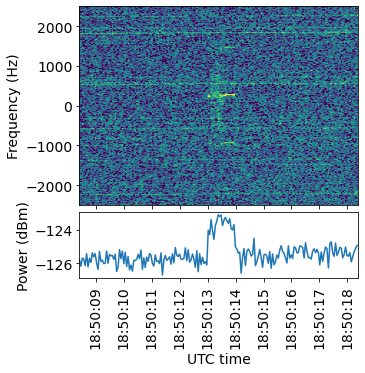
The figure below shows the waterfall corresponding to the first packet in the recording. This is the same packet that was shown above in the Inspectrum waterfall. It is also the packet with the best SNR in all the recording. A power measurement over a bandwidth of 3 kHz centred on 250 Hz (closely matching the signal bandwidth) is included below the waterfall.
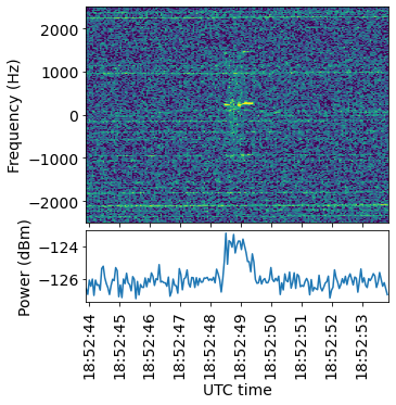
This shows another good packet. Note that in every packet the transmit frequency seems to increase slightly at the end of the packet, when the “tail” with a strong central spectral line is transmitted.
In many cases it is only possible to see this “tail” in the waterfall, since the packet is weak. The next figure also shows some of the different kinds of RFI that are present.

The Jupyter notebook contains the waterfall plots for all of the transmit periods.
Next we perform a power measurement using the first packet. To do this, we take the power measurement of the packet plus noise in the 16-bit scale and select manually the time interval where the packet is present. We average across time in the region where the packet is not present to obtain an estimate for the noise floor power. Then we subtract this estimate to obtain the power of the packet only. This is illustrated in the figure below.

Now we can compute the average power over time of the packet and use the amplitude calibration to obtain a power value in dBm. Doing so, we get -128 dBm.
To interpret this result, we compute the free space path loss. The satellite was at a distance of 6599 km when the packet was transmitted. Using this online calculator we get a free space path loss of -161.6 dB for 436.5 MHz. I don’t have an exact measurement for the gain of the Arrow antenna that I was using to receive, but since it is a 7 element yagi, its gain should be approximately 12 dBi.
Putting all of this together, we get that, ignoring any losses, the EIRP of the transmitter would be 21.6 dBm. This value will increase if we take into account losses such as polarization losses (which are not negligible by any means and could be several dB), pointing errors, cable losses, etc. I haven’t found any accurate documentation that gives the transmit power of CELESTA, but I think it is probably less than 1W. Taking the losses into account (which are probably several dB), and the fact that the transmit antenna gain could be lower than 0 dBi if we are seeing it from an unfavourable direction, the 21.6 dBm EIRP estimate that we have obtained seems a reasonable ballpark.
Code and data
The data used in this post is published as the dataset RF recording of Vega-C MEO cubesats 436 MHz telemetry beacons in Zenodo. The Jupyter notebooks and GNU Radio flowgraphs are in this repository.