Precise orbit determination for Lucky-7

In one of my previous posts, I used measurements from the GPS receiver on-board the Lucky-7 cubesat in order to find the TLE that best matched its orbit, and help determine which NORAD ID corresponded to Lucky-7.

Now I have used the same GPS measurements to perform precise orbit determination with GMAT. Here I describe the results of this experiment.

I have used a Jupyter notebook to write the GPS measurements in a tracking data file that GMAT can understand, and also to interpret and plot the results obtained with GMAT. The Lucky-7 GPS data contains ECEF positions and time (written as GPS time of week) between 14:00 and 23:00 UTC of 2019-07-22, which corresponds to approximately 5.6 orbits.

The GPS data is written to a GMAT tracking file and the following GMAT script is used to perform orbit determination. Initially, I ran this script using a state vector obtained from the TLEs, but after performing orbit determination, the result obtained can be used as initial state vector.

The force model used in GMAT intends to be as accurate as possible. It includes non-spherical Earth gravity with 360×360 EGM96 spherical harmonic coefficients, point forces for all other significant objects in the solar system, the MSISE90 atmosphere model using historical space weather taken from Celestrak, solid Earth tides, solar radiation pressure, and relativistic effects. The mass and area of Lucky-7 I have used are just crude estimates based on the fact that it is a 1U cubesat.

The GMAT script needs to be run first in orbit determination mode to produce the following estimation report. This report is then read in the Jupyter notebook in order to plot the residuals. These are shown below.

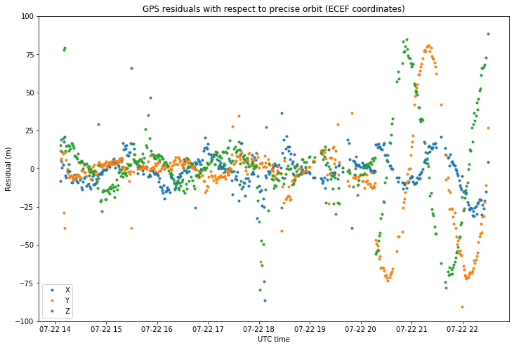
For reasons that are explained below, only the first 330 GPS measurements are considered for orbit determination. Therefore, the residuals after 20:00 UTC are much larger.

The problem with the plot of residuals shown above is that it is in ECEF coordinates, which are not so easy to interpret. It is much more useful to show the residuals in VNB coordinates, which are formed by a V vector, pointing in the direction of the velocity vector of the spacecraft, an N vector, which is normal to the orbital plane, and a B vector, which completes a right-handed orthonormal frame. The B vector lies in the orbital plane and points towards the Earth (though not exactly towards the Earth centre unless the orbit is circular).

To plot the residuals in VNB coordinates, it is necessary to run the GMAT script again in propagation mode to produce a CCSDS OEM file containing the state vector of Lucky-7 in ECI coordinates. The OEM file is then read in Python, the ECEF residuals are rotated to ECI coordinates using Astropy, and then rotated to VNB coordinates. The results are shown in the figure below.

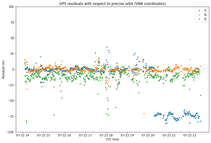
There is a very noticeable jump in the residual of the V coordinate sometime after 20:00 UTC. This is the reason why the measurements after this moment haven’t been included in the orbit determination. The jump is most likely cause by some jump in the clock of the GPS receiver on-board Lucky-7. At an orbital speed of approximately 7.5km/s, 75m corresponds to 10ms. Thus, it seems that at some point the timestamps of the GPS receiver start being 10ms earlier than they should. This is a problem with the GPS receiver. No serious GPS receiver should do this, especially if it is going to be used for orbit determination or other applications where measurement timestamping is critical.

Of course, there is no guarantee that the timestamps for the measurements before 20:00 UTC are correct either. The important point is that all the timestamps need to be consistent, meaning that they have a constant offset to UTC time. The problem here is that this offset jumps at some point.

If we zoom in the figure above, we see that the residuals for the V and N coordinates are usually smaller than 5m, which is the typical error that a GPS receiver might give. On the other hand, the residuals for the B coordinate have a much greater standard deviation and seem to be centred on -10m instead of zero.

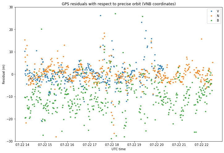
I am not sure of the reason why the B residuals are biased. The bias means that, according to the GPS measurements, the orbit is 10m higher than the precise orbit found by GMAT. Maybe this is because the drag modelling is not accurate enough.

This study has shown the possibilities of running precise orbit determination with a GPS receiver on-board a cubesat in low Earth orbit. For an interval of several revolutions, the orbit is determined with metric level precision. It would be interesting to study measurements over the course of several days to see the magnitude of the effect of orbital perturbations that are not taken into account in the GMAT force model.

Update: After some discussion on Twitter with the SkyFox Labs team, it seems that the problem with the timestamping of the GPS measurements after 20:00 UTC doesn’t have anything to do with the on-board GPS receiver, but rather with the way that the telemetry was processed on ground to produce the CSV file I used. The GPS timestamp is encoded in the Lucky-7 telemetry using 1/256th of a second units (approximately 3.9ms). Then this telemetry was processed with a Scilab script to generate the CSV file.

If we look at the fractional parts of the timestamps in the CSV file, we see that all of them are 0.64 up until some point, where they jump to 0.65. This jump of 10ms coincides with the moment when the jump in the V residual happens.

There is no possible way that the Lucky-7 telemetry has transmitted this jump, as 10ms is not an integer multiple of 1/256 seconds, so this jump must be caused by a bug in the Scilab script.

In fact, correcting the V residuals by adding them the magnitude of the velocity vector times 10ms gives the figure below, where the jump in the V component has disappeared. This shows that all the measurements where taken at a fractional part of 0.64 seconds, despite what the CSV file says.