For quite some time I’ve been thinking about generating SigMF annotations in some of the Jupyter notebooks I have about signal analysis, such as those for LTE and 5G NR. The idea is that the information about the frequencies and timestamps of the packets, as well as their type and other metadata, is already obtained in the notebook, so it is not too difficult to generate SigMF annotations with this information. The main intention is educational: the annotated SigMF file provides a visual guide that helps to understand the signal structure, and it also serves as a summary of what kind of signal detection and analysis is done in the Jupyter notebook. The code also serves as an example of how to generate annotations.
Another benefit of this idea is that it serves as a good test case for applications that display SigMF annotations. It shows what kinds of limitations the current tools have, and can also motivate new features. I’ve been toying with this idea since a while ago, but never wrote a blog post about it before. A year ago I sent a pull request to Inspectrum to be able to display annotation comments as tooltips when the mouse hovers above the annotation. While doing some tests with one LTE recording I realized that a feature like this was necessary to display any kind of detailed information about a packet. Back then, Inspectrum was the only application that was reasonably good at displaying SigMF annotations in a waterfall. Later, IQEngine has appeared as another good tool to display SigMF annotations (and also add them manually).
I have now updated the Jupyter notebook that I used to process a 5G NR downlink recording made by Benjamin Menkuec. This is much better to show an example of what I have in mind compared to the LTE recordings I was playing with before. The recording is quite short (so it is small), and I already have code to detect all the “packets”, although I have not been able to identify what kind of signals some of them are.
The modifications done to the Jupyter notebook to generate annotations are straightforward. I am using the sigmf-python library. One key idea is that all the annotations generated by the notebook use the "core:generator" key "destevez Jupyter notebook". The notebook reads the SigMF metadata at the beginning and deletes all the annotations that have this "core:generator". The rest of the code below adds annotations as packets of different types are detected and classified. This trick allows to change the code that generates the annotations and re-run the notebook to update the annotations, because the old annotations are deleted at the beginning.
I’m adding the following types of annotations:
- Frame. Identifies each radio frame, with a relative number (frame 0 is the first full frame in the recording)
- PSS. Identifies PSS symbols. The annotation comment contains the NID1 (since this information is determined by looking at the PSS).
- SSS. Identifies SSS symbols. The annotation comment contains the NID1, NID2 and cell ID (since this information is determined by looking at the SSS after the PSS has been processed).
- PBCH. Identifies the PBCH symbols. The annotation comment contains the cell ID and the Issb index, since that information is necessary to generate the PBCH DMRS. In the notebook I’m not decoding and parsing the PBCH (I did this for LTE in this post), but if I were, I could also add the PBCH fields to the annotation comment.
- PDCCH. Identifies PDCCH symbols.
- PDSCH and PDSCH DM-RS. The PDSCH annotation identifies the full PDSCH transmission (composed of 9 data symbols and 3 DM-RS symbols). Each PDSCH DM-RS annotation identifies a single DM-RS symbol. These give a good example of overlapping annotations to test how applications behave, since the PDSCH DM-RS annotations are fully contained inside the PDSCH annotation. Since Inspectrum always displays the annotation label, in the PDSCH DM-RS annotations there is no label to avoid clutter. The comment of these contains “PDSCH DM-RS”, which should be visible as a tooltip on mouseover.
- There are other signals in the recording that I have not identified. These are marked with a ??? annotation. The comment contains some additional information, such as “Only every 12th subcarrier is active”.
The SigMF file can be found in this folder. A recent enough version of Inspectrum needs to be used to display SigMF annotations. Luckily, all the pull requests that I have sent as part of my experiments are available in Inspectrum v0.3.1, released in October after several years without tagged releases.
The screenshot below shows how Inspectrum displays the annotations in the busiest part of the recording. This is the subframe in which the SIB1 is transmitted, which is done using the PDSCH, which in turn needs a PDCCH transmission. In comparsion, most other subframes in this recording of an idle srsRAN gNB are mostly empty.
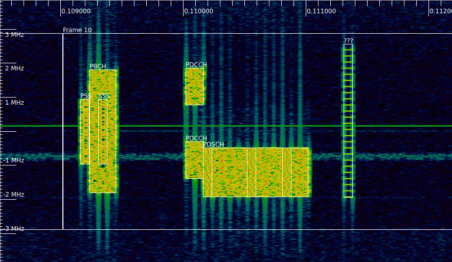
It is easy to adjust the FFT size and time zoom to be able to see the annotations well. The placement of the bounding boxes and labels is good, even for the SSS, which is inside the PBCH.
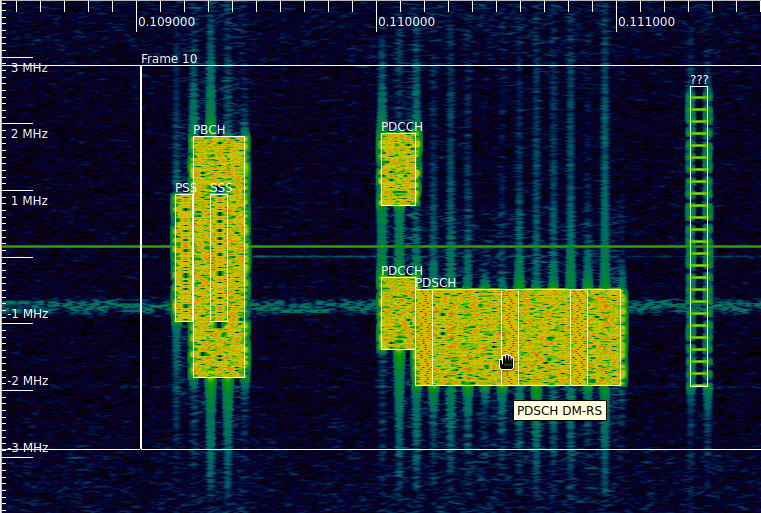
The next screenshot shows an example of a mouseover tooltip showing an annotation comment (in this case identifying the PDSCH DM-RS). To make this work, I sent a pull request that checks if any of the overlapping annotations below the cursor has a comment, and displays that as a tooltip. If several overlapping annotations have a comment, only one of them is shown. In this case, this gives problems for the SSS. Its comment is never shown, since the PBCH comment is shown instead. This example shows that when we consider overlapping annotations there are many corner cases in which it is not even clear what is the best approach.
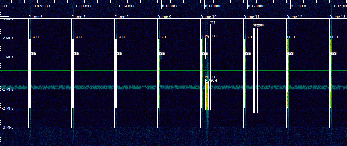
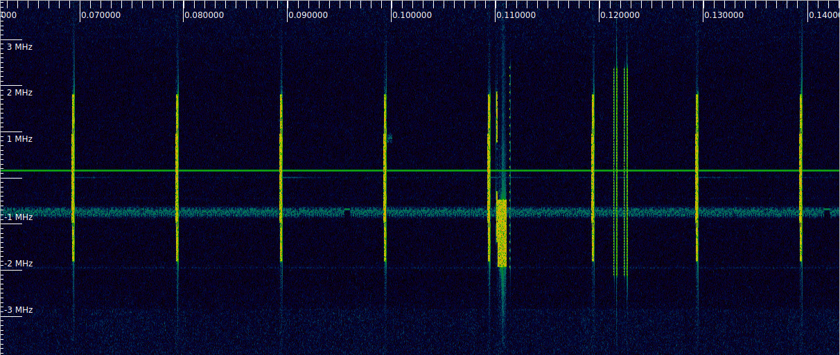
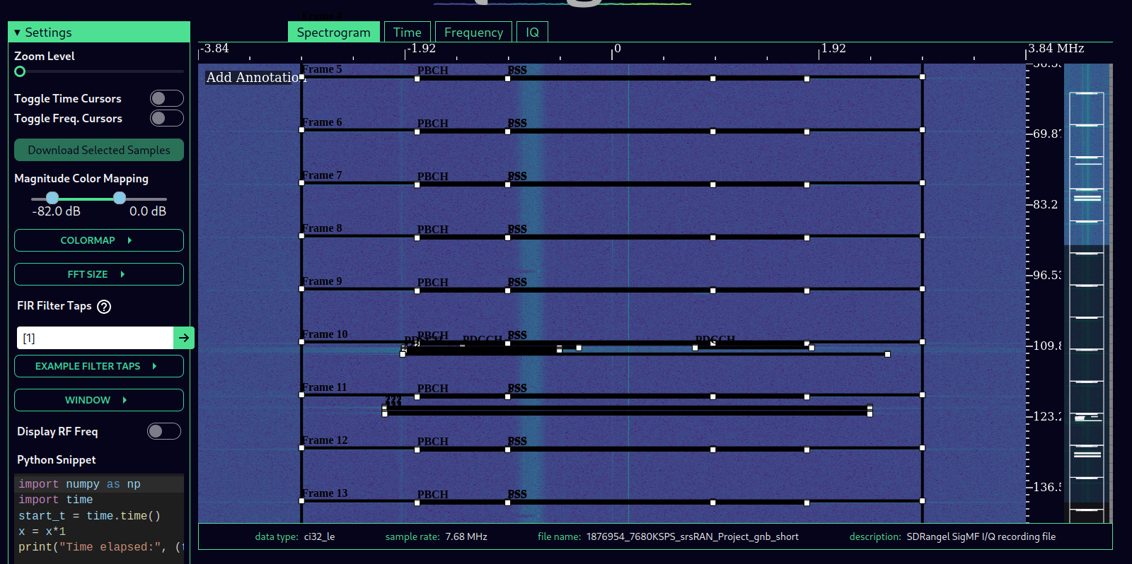
Zooming all the way out gives a good overview of the recording. It shows the PBCH at the beginning of each radio frame, and it also shows which frames have some other signals. At this zoom level the annotation boxes almost hide the waterfall, so it is good to click the Display Annotations checkbox (conveniently located in the left panel) to toggle between annotations on and off to see the waterfall better (second plot).
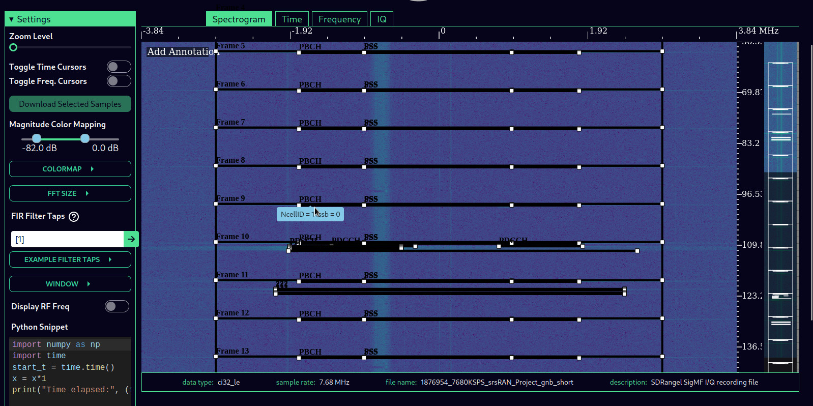
The SigMF file can be viewed in IQEngine by using the Local File Browser option to load it from disk. The default view works well as an overview of the recording, in the same way as the previous Inspectrum screenshot. However, it doesn’t seem possible to zoom in more in time (the Zoom level slider zooms out instead) or to hide the annotations.
Annotation comments are shown as a tooltip on mouseover, in the same way as in Inspectrum. However, newline characters are replaced by a space, which would make longer multiline text more difficult to read. Due to the zoom limitation, I haven’t been able to test how tooltips for overlapping annotations work. The mouseover seems to happen when hovering over the label instead of the bounding box, which might be a good idea to handle overlaps (because it’s less likely to have overlapping labels).
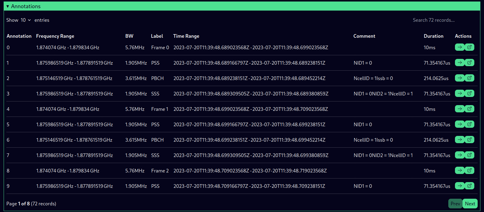
A nice IQEngine feature that Inspectrum doesn’t have is a list of all the annotations in the file. Annotations can be selected and even any annotation field can be edited using this list. At least for the use cases I have in mind, the frequency range, time range and duration fields show too many decimals, and the comment field is too narrow and removes newline characters. There is even a search field, but I doesn’t seem to work (I’m testing this with Firefox 116.0.3; maybe it works with Chrome).
What is beyond all of this? I dream of being able to introduce other information in the SigMF annotations and have applications display it. For example, constellation plots. I have plenty of those in my notebooks. It would be awesome to be able to include them in the SigMF metadata and browse through them interactively. Currently there is no standard way to do this with SigMF, though it is possible to define a custom extension that includes the constellation plot as an image in base64 (or maybe a list of complex symbols, though that places the burden of formatting the plot in the visualization application). There are also many good design questions about how a UI that can display this kind of data should look like.
My idea is to have SigMF files whose annotations are as rich as possible, containing anything one could think of about each packet: SNR and other scalar estimates obtained by the receiver, constellation plot, data contents parsed according to the protocol, etc. To list a few short sentences, the comment field is good for now, but it is not good for adding a lot of data, such as parsed packet payload. Nevertheless the problem in all generality is a daunting task, because there are many different radio protocols and properties that can be measured, so I just wanted to pique the interest with these ideas.