Back in March, I was helping Julien Nicolas F4HVX to test the S-band image transmitter of AMICal Sat before launch. In my post back then, I explained that AMICal Sat uses a Nordic Semiconductor nRF24L01+ 2.4GHz FSK transceiver chip to transmit Shockburst packets at 1Mbaud. I also explained how the Onyx EV76C664 CMOS image sensor works and how to process raw images.
AMICal Sat was finally launched on 2020-09-03, and since them the satellite team has been busy trying to downlink some images, both using the UHF transmitter (which uses the same protocol as Światowid) and the S-band transmitter. This has proven a bit difficult because the ADCS of the satellite is not working, and the downlink protocols are not very robust.
Julien has been sending me recordings done by their groundstation in Russia with the hope that we could be able to decode some of the data. Before several failed attempts where we were hardly able to decode a few packets, we got a particularly good S-band recording done on 2020-10-05. Using that recording, I have been able to decode a full image.
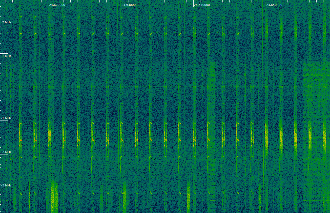
The recording is a 7.5Msps IQ recording that lasts for about 65 seconds. The frequencies in the recording are inverted, as one can check by examining the AMICal Sat Shockburst frames and noting that the characteristic 0xe7e7e7e7e7 address in inverted. Therefore, it is necessary to invert the frequencies by taking the complex conjugate or swapping I and Q before continuing. I don’t know the centre frequency of the recording, but the AMICal Sat signal can be found at -1.55MHz in the original recording.
Below we can see one of the Shockburst packets from the recording being FM demodulated in inspectrum. Note that there is a huge frequency drift at the beginning of the packet. Luckily, by the time that the 0xe7e7e7e7e address starts (which is what I use for frame synchronization), the frequency is already settling.

In hindsight, this frequency drift problem was already present in the pre-flight recordings we used in March. This, together with the lack of a moderately long preamble in Shockburst packets is what made me spend some time tuning an FSK demodulator for these short bursts.
The decoder that I have used is basically the same GNU Radio flowgraph to decode Shockburst packets that I used in March. It can be obtained here. The flowgraph saves all the frames that have a 0xe7e7e7e7e7 address with no bit errors into a file, regardless of whether the CRC is correct. Several copies of each frame are usually stored in the file, since there are multiple decoders in parallel trying different clock phases.
The Shockburst packets are then analyzed in this Jupyter notebook, which I have adapted from my work in March. First we filter out the frames having incorrect CRC-16. The first 2 bytes of each packet (after the address) contain a frame counter that increases starting from zero to indicate which chunk of the file is being transmitted.
The value of this field is shown in the figure below. The large spikes correspond to packets whose frame count field contains 0x5555. These packets are special and seem to indicate that a file downlink is starting. We see that after these packets the frame counter starts from zero and keeps increasing until the whole file is transmitted, and then gets back to zero as a new transmission starts.

There are five transmissions in total, which are separated by a gap of several seconds with no signal. The file sent in each of the transmissions is actually the same one. By sending the same file multiple times, the chances of successfully receiving all the frames are maximized.
The special packets that contain 0x5555 in their frame count field are all the same and contain the following payload (not including the CRC-16):
55555555555555555555555555555555555555555555555555555555a0760000
They are very easy to see in the spectrum, due to the long string of 0x55 bytes and the lack of a scrambler. Note that we don’t have special packets between the first and second transmission. This is just because we haven’t been able to decode any of these special packets correctly, as they are clearly present in the recording.
The figure below shows the start of the transmission (WiFi interference included). We see 17 of these special packets, which show a strong carrier, and then the regular packets containing the file chunks.
I have put together some code that assembles a file by using the frame count and detects the number of missing packets that were skipped. When we treat each transmission individually, we obtain the following:
Skipped 15 / 948 frames
Skipped 30 / 948 frames
Skipped 25 / 948 frames
Skipped 26 / 948 frames
Skipped 37 / 948 frames
We see that there is a frame loss of around 2.5%. However, when we take into account that these are five repetitions of the same file, we can put together the whole file without any missing frames. The file has 28470 bytes and can be downloaded here.
As I explained in my post in March, the start of the file has a 512 byte header with metadata. I have made a Jupyter notebook to parse the metadata according to the table I showed in that post. However, I have needed to make some minor modifications to the fields by adding a couple of padding fields that were not present in the table. Julien has helped me with this by showing me the metadata values obtained with the software that the team is using. The padding fields are quite easy to spot because they contain 0xaa bytes. The contents of the metadata header are as follows:
Container:
    timestamp = 1601326224
    set_point = ListContainer:
        -3.0316488252093987e-13
        -3.0316488252093987e-13
        -3.0316488252093987e-13
        -3.0316488252093987e-13
    estimated_point = ListContainer:
        -3.0316488252093987e-13
        -3.0316488252093987e-13
        -3.0316488252093987e-13
        -3.0316488252093987e-13
    lat_lon = ListContainer:
        -3.0316488252093987e-13
        -3.0316488252093987e-13
    gyroscope = ListContainer:
        43690
        43690
        43690
    magnetometer = ListContainer:
        43690
        43690
        43690
    earth_magnetic_model = ListContainer:
        43690
        43690
        43690
        43690
        43690
    sun_sensor = ListContainer:
        43690
        43690
    pixel_resolution = 8
    compression = 1
    dummy0 = b'\xaa\xaa' (total 2)
    picture_size = 27934
    sensor_gains = ListContainer:
        64
        32896
        32896
        0
        1920
    dummy1 = b'\xaa\xaa' (total 2)
    exposure_time = 1000000
    sensor_temperature = 223
    dummy = b'\xaa\xaa\xaa\xaa\xaa\xaa\xaa\xaa\xaa\xaa\xaa\xaa\xaa\xaa\xaa\xaa'... (truncated, total 412)
    crc = 10481
The timestamp seems correct and is the UNIX timestamp for 2020-09-28 20:50:25, which I guess makes sense. Most of the fields don’t contain valid data, presumably because the ADCS system is not working.
The rest of the file contains a raw image compressed with the fpaq0f2 algorithm. The fpaq0f2 software is a simple C++ program. The file can be decompressed like so:
$ tail -c +513 compressed_image_with_header > compressed_image_no_header
$ g++ -o fpaq0f2 fpaq0f2.c
$ ./fpaq0f2 d compressed_image_no_header raw_image
compressed_image_no_header (27937 bytes) -> raw_image (1441792 bytes) in 0.46 s.
The raw image we obtain is a 704×1024 pixel 12 bit image. Each pixel value is stored as a little-endian uint16_t, and the sparse colour pixel arrangement of the sensor follows what I described in my post from March. It is interesting that the horizontal resolution has been decimated by 2. The full images from the sensor are 1408×1024, of which only the leftmost 1280 columns are usable.
After running the image through my code that converts it to an RGB image, we obtain the following.

There is not much to see here. The band on the right is the unusable area of the image, and looks the same as in those images taken in the lab in March, but with many hot pixels, especially in the bottom. The usable area of the image is very dark, but there are a few pixels that are brighter than the rest. We can exaggerate this by pretending that the image is 9 bits depth instead of 12, so anything having a value of more than 1/8th full scale will saturate.
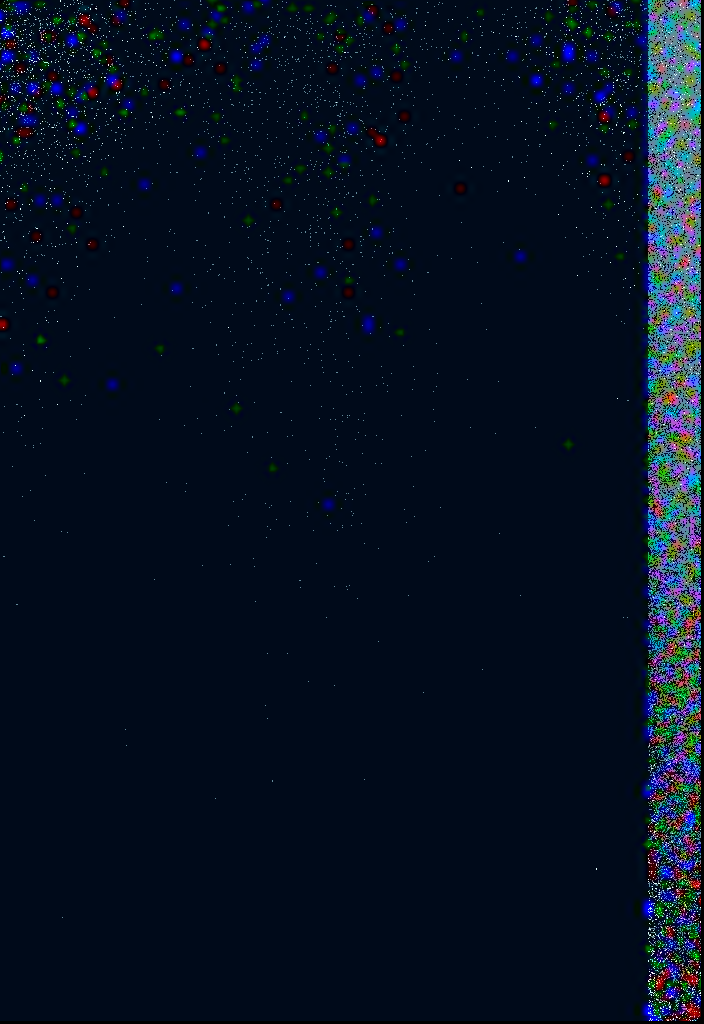
Note that colour pixels (especially blue and red) have an effect over a relatively large area of the image and show up as a small blob rather than a dot. This is just because the resolution of the blue and red pixels is 1/8th of the total resolution (in both the vertical and horizontal directions), so the value of these pixels is assigned to the small area of 8×8 pixels surrounding them (I’m actually oversimplifying the image processing algorithm to explain this).
It is also interesting to look at the raw pixel values, shown below.
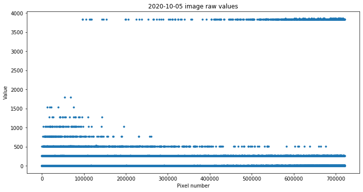
Some of the values are quite near the full scale of 4095. I think these correspond to hot pixels that are either dead or perhaps affected by radiation when the image was taken. The other values seem to cluster around multiples of 256, which is quite surprising. I don’t know what could cause this.
We can study this in more detail in the following histogram, which shows the relative proportion in which the different pixel values appear. Note that the vertical scale is logarithmic (in fact most of the pixels have the value 0, so we would see nothing in a linear scale), and that the horizontal axis has jumps (we jump from 15 to 256, for instance). These are all the pixel values that appear in the image. It is surprising that there are relatively few, rather than having values spread over a continuum.

The image processing code can be found in this Jupyter notebook. Currently the satellite team is studying this image in more detail to see what else can be learned from it. Best of luck to the AMICal Sat team with their mission.
Update 2020-10-12: Julien has made me notice that the raw image is actually 8 bits depth stored as uint8_t, rather than 12 bits stored as uint16_t. This explains why I thought that the horizontal resolution was 704 pixels, half the normal of 1408 pixels. It also explains the clustering of values around multiples of 256. In fact, the most-significant-byte of each uint16_t was actually the value of another pixel.
With this in mind, I have updated the notebook. The image is now as follows.

As we can see in the histogram below, all the pixel values are below 16, from a possible maximum of 255. In fact, most “hot pixels” are 15, while it would make sense for them to be 255.
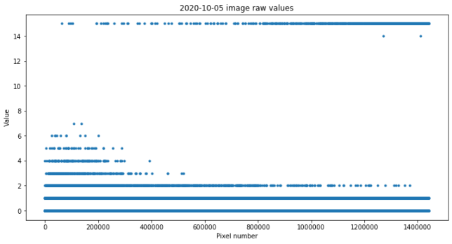
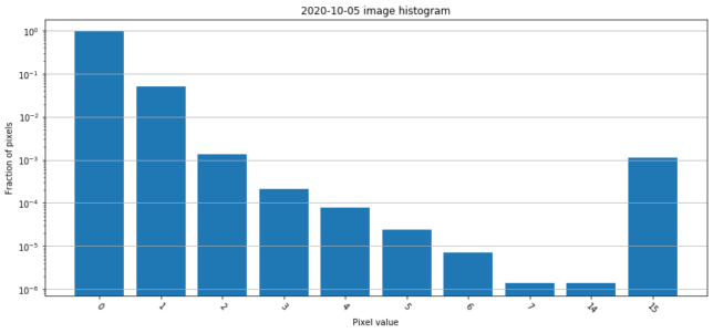
I’m guessing that maybe the conversion from 12 bits to 8 bits is not correctly implemented, and leaves only 4 valid bits. Rescaling the values as if it was a 4 bit image, we obtain the image below. Now the band on the right is visible and has the same aspect as in the pre-flight images done in the lab.

In fact, most of the pixel values in this band on the right are 1. On the 12 bit images done in the lab the values in this band were around 200. Therefore, after a division by 16 to pass to 8 bits, we would expect values around 12. However, if instead we do a rounded division by 256, then we get 1. This supports my idea that the image has been inadvertently left with only 4 bits of depth.