AMICal Sat is a 2U cubesat developed by the Space Centre of the Grenoble University, France, and the Skobeltsyn Institute of Nuclear Physics in the Lomonosov Moscow State University. Its scientific mission consists in taking images of auroras from low Earth orbit. The satellite bus was built by SatRevolution. Currently, the satellite is in Grenoble waiting to be launched on a future date (which is uncertain due to the COVID-19 situation).
A few weeks ago I was working with Julien Nicolas F4HVX to try to decode some of the images transmitted by AMICal Sat. Julien is an Amateur radio operator and he is helping the satellite team at Grenoble with the communications of the satellite.
This post is an account of our progress so far.
AMICal Sat has a UHF transmitter for the 70cm Amateur satellite band and an S-band transmitter for the 2.4GHz Amateur satellite band. The UHF transmitter uses 9k6 FSK and can transmit images using a protocol similar to the one used by Światowid. The S-band transmitter is a high-speed transmitter, so it is desirable to use it as the main transmitter for the high resolution scientific images taken by the payload, leaving the UHF transmitter as a backup. Julien and I have been working with the S-band transmitter, so in this post I won’t speak about the UHF transmitter.
S-band packets
The S-band transmitter is based on a Nordic Semiconductor nRF24L01+ 2.4GHz FSK transceiver chip (see the datasheet here). The images are sent in 1Mbaud GFSK Shockburst packets. The structure of a Shockburst packet can be seen in the figure below, taken from the nRF24L01+ datasheet.
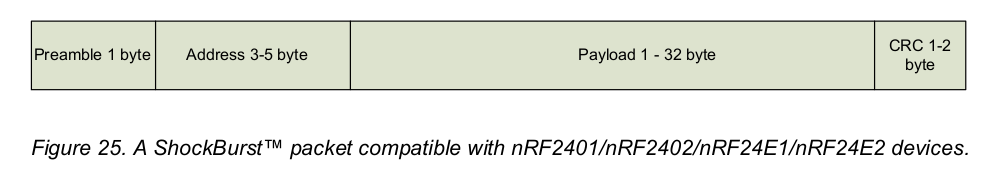
AMICal Sat uses the 5 byte address 0xe7e7e7e7e7, a 32 byte payload, and a 2 byte CRC. The CRC used by ShockBurst is the one called CRC_CCITT_FALSE in this online calculator, and covers both the address and the payload. The payload of each packet consists of a chunk counter, which is a 16-bit little endian integer, followed by a 30 byte chunk of the image file.
The image file has a 512 byte header followed by the image data. The header is described by the table below (all the fields are little endian).
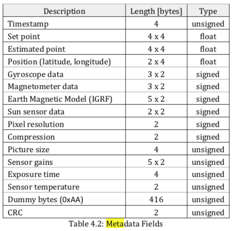
The image data can be sent either uncompressed or compressed with fpaq0f2.
The main difficulty we’ve been facing is decoding all the packets without any bit errors. Even though Julien has made IQ recordings of the satellite in the lab, and the SNR is more or less good, it seems extremely difficult not to lose any packets due to bit errors.
In an attempt to reduced the errors, I have tried hard to design a reliable decoder in GNU Radio. The main ideas of this decoder are as follows. First, no clock recovery is done. This is acceptable, since the packets are rather short, and it increases reliability, as it eliminates the clock recovery loop as a possible point of failure. Four different clock phases are tried in parallel and packets decodes from all of them are stored for later processing.
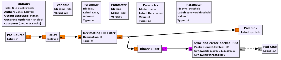
Second, there are two different decoding algorithms which are tried in parallel. The first one is an integrate and dump FSK demodulation algorithm. This is best explained by the diagram below, taken from this post in David Rowe VK5DGR’s blog.
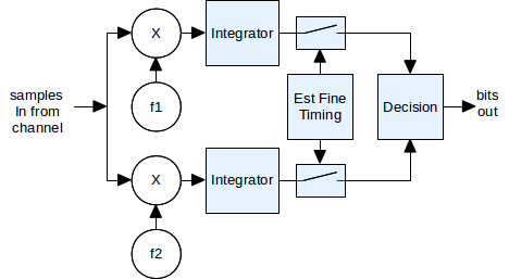
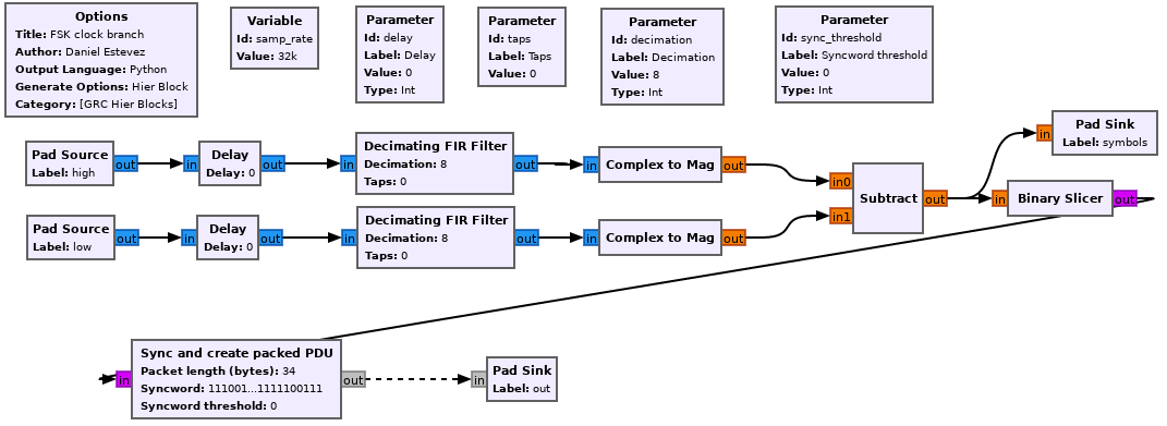
Essentially, each of the FSK tones is shifted to baseband, integrated coherently for a bit period, and then power is compared. This demodulator is implemented as a hierarchical flowgraph, which is instanced for each of the four clock phases. The flowgraph is shown in the figure below. The Sync and create packed PDU block from gr-satellites is used to detect the address and extract the payload and CRC as a PDU.
The second decoding algorithm is based on FM demodulation, followed by some filtering and bit slicing.
The full decoder can be seen in the figure below. There are four instances of the integrate and dump demodulator (called FSK clock branch) and four instances of the FM-based demodulator (called NRZ clock branch). Packets decoded from any of the branches are stored in a file for later processing.
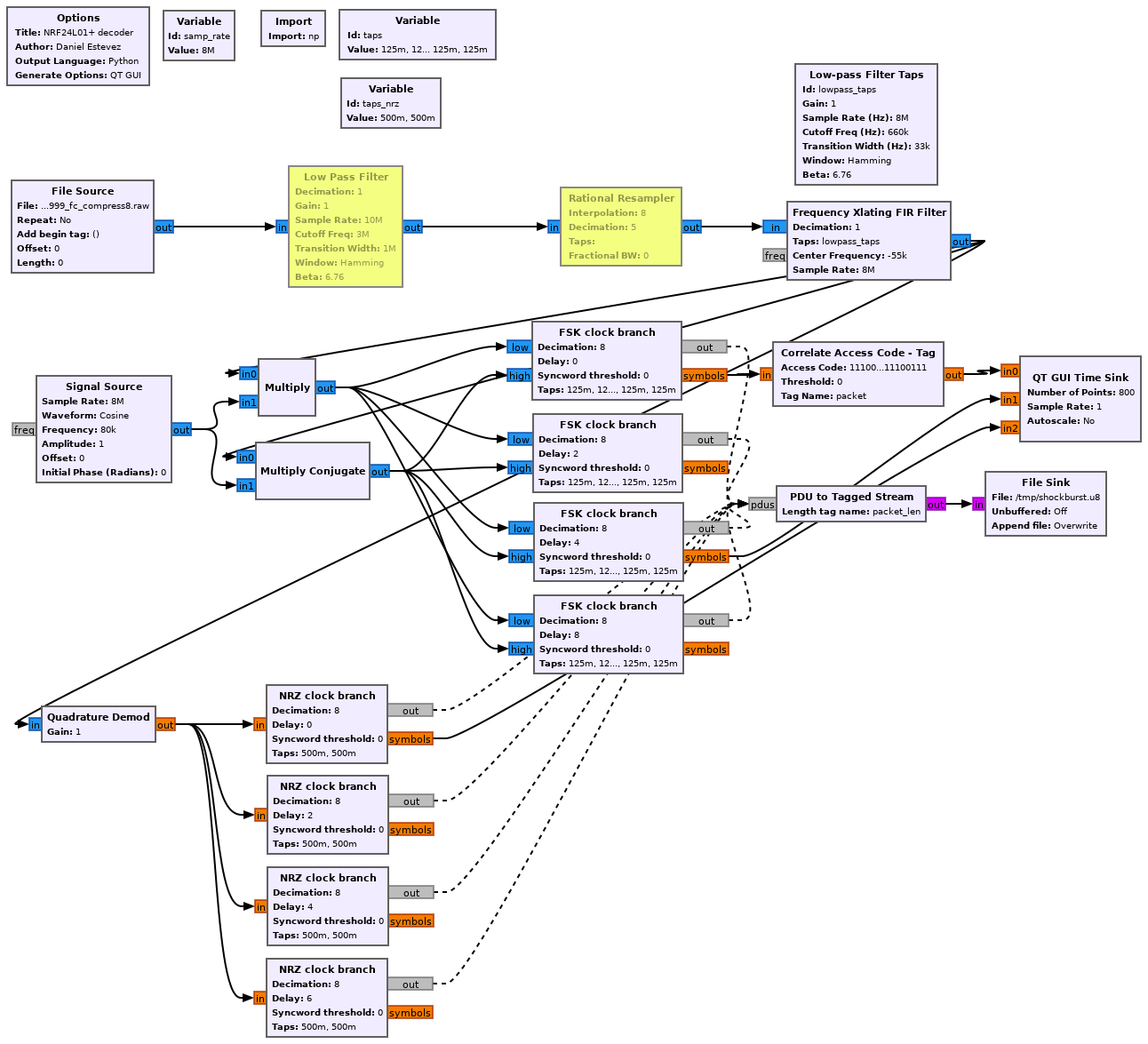
The decoder flowgraph can be found in nrf24.grc.
After decoding, the frames are processed in this Jupyter notebook. It performs CRC checking, dropping all messages with invalid CRC. The remaining messages are grouped according to their chunk counter (first 2 bytes of the payload).
Ideally, we would expect that all the frames with the same chunk counter and correct CRC are equal (they are just the same frame decoded in parallel successfully by several of the eight demodulators). However, due to the short length of the CRC-16 code, we see many corrupted frames with valid CRC. To solve this problem, for each chunk counter value, a majority voting among the frames with that particular chunk counter value and correct CRC is done to try to select the correct frame. Often, the frame is decoded correctly by several of the eight demodulators, so this majority voting approach seems to work well to discard corrupted frames.
According to the result of the majority voting, the image file is reassembled using the chunk counter of each frame. Any missing frame leaves a gap of 30 bytes of zeros in the file.
Even after all this work, we haven’t managed to decode a transmission without any errors. The number of lost frames we get is quite low (on the order of 1%), but to recover compressed images we need perfect decoding, as any gaps in the file will make the decompression algorithm fail.
Image data
The image sensor used by AMICal Sat is an Onyx EV76C664 1280×1024 pixel sparse colour CMOS sensor. This means that whereas in most sensors the colour filter array has mainly coloured pixels, in this sensor most of the pixels are white, as shown by the figure below, taken from the datasheet.
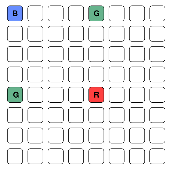
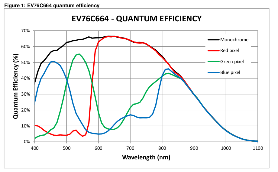
I don’t know much about image sensors, but the manufacturer claims that this gives the sensor better low-light performance, which seems reasonable and is very desirable for AMICal Sat use case. The figure below, also taken from the datasheet, helps illustrate the advantage of having many white pixels.
The sensor active area is 1408×1040 pixels, with a useful area of 1280×1024 pixels. The ADC has 14 bit depth, but often a lower depth, such as 12 or 10 bits is used.
The image sensor data can be sent as uncompressed raw ADC data or as raw ADC data compressed with fpaq0f2. We haven’t been able to decode a compressed image successfully, due to packet loss, but we have managed to put together some uncompressed images.
Raw ADC data is sent as little endian 16 bit integers scanning the full 1408×1040 sensor area. In these integers, only the 12 or 10 least significant bits are nonzero, depending on the image depth. Decoding of the raw data is done in this Jupyter notebook.
I don’t usually work with colour image data, so my background read on colour spaces and human colour perception has been quite interesting. To decode the image, first each of the R, G, B and Y (luminance, from white pixes) channels are extracted and interpolated to the full sensor size. Then, the chroma information in the RGB channels is converted to CbCr using the JPEG conversion. A translation is done in CbCr coordinates for white calibration (the appropriate translation has been determined experimentally with a calibration image). Finally, the CbCr information is taken together with the Y channel from white pixels and converted back to RGB. Note that this is a very naïve demosaicing algorithm and, specially given the low chroma resolution, gives suboptimal results.
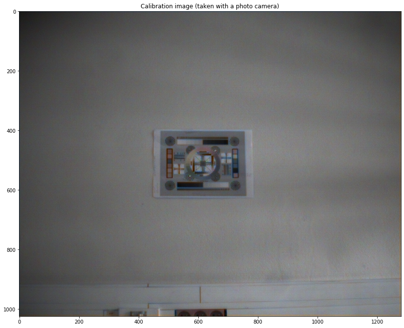
The first raw images I have worked with are a couple of calibration images taken in the lab. These are images of a calibration sheet taken at 12 and 10 bit depth. For some reason, the raw images have already been cropped to the 1280×1024 sensor useful size.
The figure below shows the calibration sheet photographed with a regular camera, for reference.
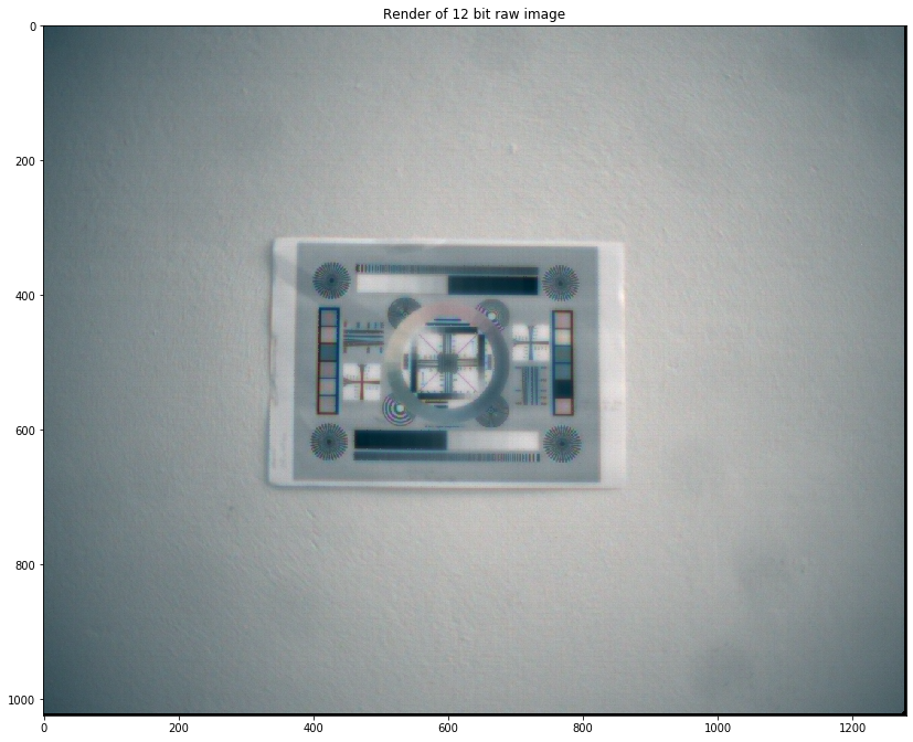
Below we show the image of the calibration sheet rendered from a 12 bit raw image taken with the AMICal Sat camera.
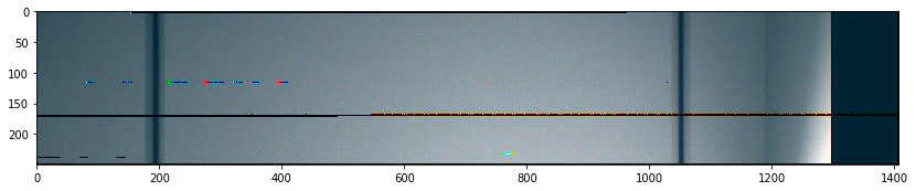
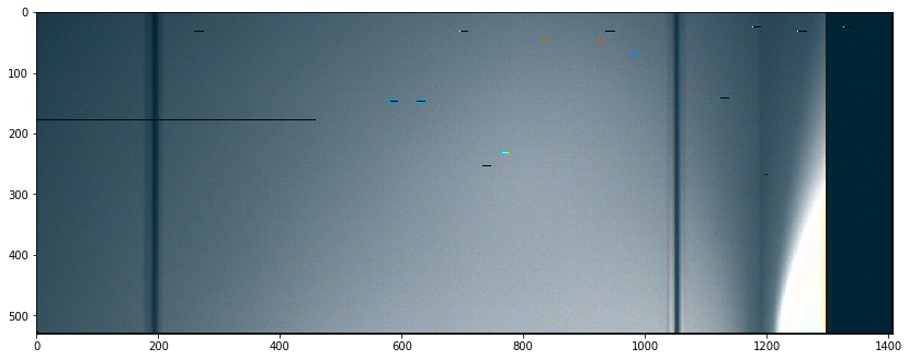
The two images below have been recovered from IQ recordings that Julien made of the S-band transmitter. The packet loss is apparent as black lines or very bright colours in some parts of the images. The data is 1408 columns wide, corresponding to the full sensor size. The useless sensor area can be seen as a dark stripe in the right side of the image. These images may not seem like much, but Julien tells me that they look like the corner in AMICal Sat’s clean room, so it seems all our software is working correctly.
It is interesting to look at the useless sensor area on the right side of the image. For some reason, it is only 112 pixels wide, even though there are 128 useless pixels per row, according to the sensor datasheet. The figure below shows the histogram for the raw ADC values corresponding to these pixels. The data seems normally distributed with small variance, as if the ADC was held to a fixed voltage or left floating.
If we average the data by columns, it seems that there is a slight variation from left to right. Note that the variation is only around 3 ADC counts, while the standard deviation of the pixel values is 5.4 ADC counts, so averaging is needed to see this effect clearly. I don’t know anything about its cause.
One comment