Voyager-1 single dish detection at Allen Telescope Array

This post has been delayed by several months, as some other things (like Chang’e 5) kept getting in the way. As part of the GNU Radio activities in Allen Telescope Array, on 14 November 2020 we tried to detect the X-band signal of Voyager-1, which at that time was at a distance of 151.72 au (22697 millions of km) from Earth. After analysing the recorded IQ data to carefully correct for Doppler and stack up all the signal power, I published in Twitter the news that the signal could clearly be seen in some of the recordings.

Since then, I have been intending to write a post explaining in detail the signal processing and publishing the recorded data. I must add that detecting Voyager-1 with ATA was a significant feat. Since November, we have attempted to detect Voyager-1 again on another occasion, using the same signal processing pipeline, without any luck. Since in the optimal conditions the signal is already very weak, it has to be ensured that all the equipment is working properly. Problems are difficult to debug, because any issue will typically impede successful detection, without giving an indication of what went wrong.

I have published the IQ recordings of this observation in the following datasets in Zenodo:

• Voyager-1 recording with Allen Telescope Array on 2020-11-14: scan 1/4
• Voyager-1 recording with Allen Telescope Array on 2020-11-14: scan 2/4
• Voyager-1 recording with Allen Telescope Array on 2020-11-14: scan 3/4
• Voyager-1 recording with Allen Telescope Array on 2020-11-14: scan 4/4

Observation set up

The observation was done between 18:30 and 21:30 UTC on 2020-11-14, when Voyager-1 was between 40 and 60 degrees elevation. Antennas 1a and 4g were used. These are two antennas having the older feeds described in this paper, which have lower performance at X-band than the newer feeds donated by Franklin Antonio, which are described here. The reason for choosing antennas with older feeds was to have two antennas having the same feed type, as that might simplify calibration for beamforming (which would become necessary if the signal was too weak to be detected with a single dish). At that time we only had access to antenna 4g with one of the USRPs used by the GNU Radio team, so we chose a matching older feed antenna to use with the other USRP.

The dual polarization signals from the antennas were taken to LO d in the RF converter board, which converted from 8419.7 MHz down to an IF of 512 MHz. The IF was received and digitised with a USRP N321 and a USRP N320. The two X and Y polarizations of antenna 1a were routed to the two channels of the USRP N321, and the two polarizations of antenna 4g were received with the USRP N320. The LO of the first channel of the USRP N321 was exported and shared to all the other channels. GNU Radio was used to record synchronized baseband IQ data from the two USRPs at a sample rate of 960 ksps using int16 format.

In order to make beamforming possible later on with the recordings, interferometric observations of the compact calibrator 1733-130 were done. This source appears in the list of VLA calibrators, and it was near the position of Voyager-1 on the sky. These observations would allow us to calibrate the phase offsets between the two antennas if needed for beamforming.

The observation was organized as four 30 minute scans of Voyager-1 interleaved with 5 minute scans of the calibrator. Longer scans of the calibrator were done before and after the four scans of Voyager-1.

Signal processing

The signal processing of the IQ recordings is done in this Jupyter notebook, which can be found in my ata_notebooks Github repository.

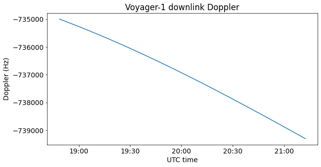
The first step is to fetch the ephemeris data from JPL HORIZONS using Astroquery. I learned this library from Nick Foster, who has a similar Jupyter notebook to process Voyager-1 recordings done with ATA on 2010. We need the range-rate from the ephemerides in order to compute and correct for the downlink Doppler, which is shown below.

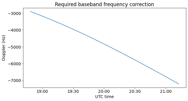
The a priori estimate for the spacecraft’s transmit frequency was 8420.432097 MHz. In order to take the downlink Doppler into account, the recording was centred at 8419.7 MHz, as mentioned above. The residual Doppler that should appear in the baseband data is as follows.

The signal will be detected in a sub-Hz FFT resolution bandwidth, so we want our Doppler correction calculations to have precision of mHz. Therefore, the range-rate data is fetched from Horizons in steps of approximately 8.6 seconds and linearly interpolated to a grid with 10 ms spacing. The carrier phase corresponding to the integrated Doppler is computed over this 10 ms grid.

Dask is used for parallel computation and on demand loading of the IQ data by chunks. Each of the 30 minute scans is processed separately. The first step in the signal processing chain amounts to removing the DC spike. This is done by grouping the samples in segments of approximately 0.5 seconds and subtracting from each segment its average.

Next, the average power per channel over all the 30 minute scan is computed. Each channel is divided by its average power in order to normalize the power, since each channel has different amplitude gains. Then, LHCP and RHCP polarizations are synthesised from the linear X and Y polarizations. To do so, the phase offset between the X and Y channels of each antenna is needed. These phase offsets were measured by receiving the RHCP X-band signal from Tianwen-1 at 8431 MHz earlier that day. The phase offsets are assumed to be the same at the receive frequency for Voyager-1.

The phase for Doppler correction is linearly interpolated from its 10 ms grid to each sample and applied in order to correct for Doppler. Finally, an FFT with a bin size of 458 mHz, rectangular window and no overlaps is applied to the data and average power spectral densities are computed per antenna, polarization and scan.

Results

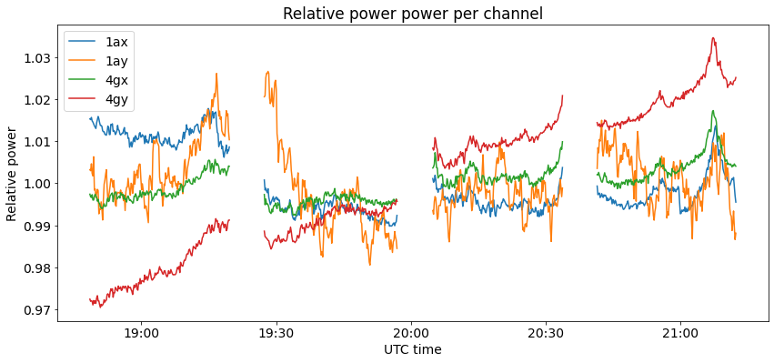
A preliminary step to assess the quality of the IQ recordings is to plot the power of each channel versus time. Since the signal is tiny in the 960 kHz bandwidth, this gives basically the power of the noise floor, which can change due to changes in gain, noise figure, interference, etc. Plotting the power can help us spot any obvious problems such as the sudden increases in the noise floor that we are seeing with some of the Chang’e 5 recordings.

Since each of the channels has a different gain, we normalize the power in each channel by dividing by the average power of that channel computed over all the four scans. This makes the power be centred about one, and gives the figure below. We see that the power variation is only of a few percent, so everything seems alright.

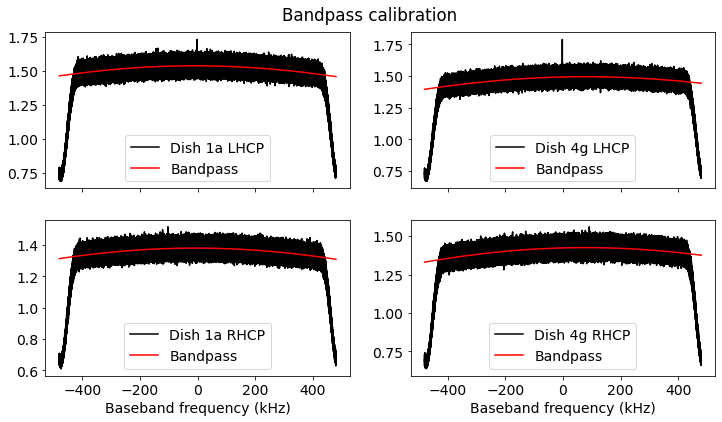
The first step in processing the Doppler corrected spectra is to perform a bandpass calibration to flatten out the bandpass frequency response. This is done by fitting a degree four polynomial to the average spectra of each antenna and polarization (ignoring the steep skirts at the edges). The figure below shows the uncorrected spectra and the estimated bandpass shape. The peak of the Voyager-1 signal can already be seen clearly in the LHCP signal from antenna 4g, and also in antenna 1a, albeit a bit weaker.

The bandpass calibrated spectra are show below.

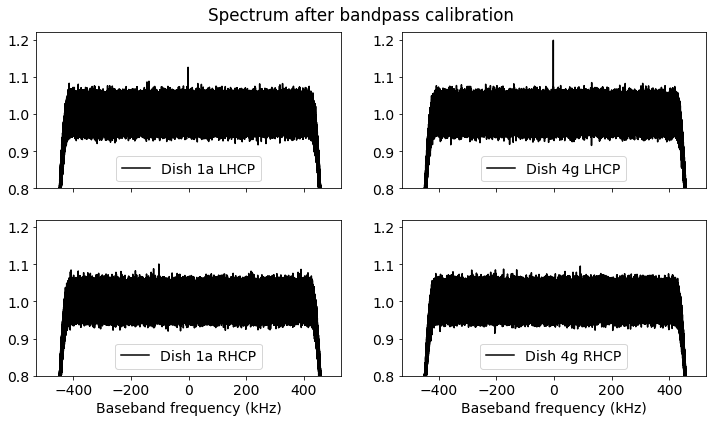
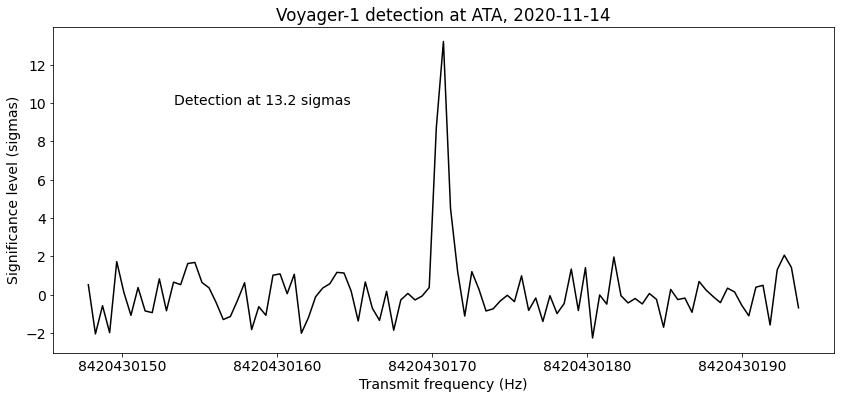
The average power spectral density for the LHCP polarizations between both antennas is computed and transformed to significance level (units of sigmas) by subtracting one, which is the average noise power, and dividing by the standard deviation. We get the figure below, which shows a detection at a level of 13.2 sigmas at a transmit frequency of 8420430170.7 Hz. This frequency is close to the a priori expected transmit frequency, so we are confident that this detection is in fact the Voyager-1 carrier. Moreover, if the Doppler correction is disabled, the detection peak disappears completely.

The next figure shows the power spectra in each of the antennas and polarizations per scan. We see that there is a clear peak in the first two scans, the peak is weaker in the third one, and disappears in the last scan. The reason why the SNR decreases throughout the observation is not known.

The estimates of C/N0 for the first two scans are given in the table below. These should be taken carefully. They are coarse estimates, since the signal is weak. The C/N0’s for the last two scans are not given, since the signal is already too weak.

	Antenna 1a	Antenna 4g
First scan	-8.5 dB·Hz	-6.4 dB·Hz
Second Scan	-8.8 dB·Hz	-6.7 dB·Hz

There seems to be a difference in performance of 2.1 dB between antennas 1a and 4g that needs to be investigated further.

Conclusions

Doing a link budget for Voyager-1 is not so easy, since we don’t have an accurate estimate of its transmit power. Perhaps, it’s better to work with the estimated received power shown in NASA DSN Now, which is around -156 dBm for a 70 m antenna (under bad weather conditions, the signal may drop to -161 dBm, as shown by Richard Stephenson in this tweet). Assuming the same efficiency, one of the ATA 6.1 m antennas should receive a power of -177.2 dBm. At a system noise temperature of 60 K (which is taken from this paper but perhaps too optimistic), the noise floor is at -181 dBm/Hz, so we should find the carrier at a CN0 of 3.8 dB.

It seems that the CN0 we measured is 10 dB below this estimate, so either there is something wrong with the estimate or there is room for improvement with the receive chain at ATA. This is something that we’ll need to look into in the future, by measuring the performance of the system in terms of noise figure, gain, etc.

Nevertheless, we have shown that it’s possible to detect with the current equipment the Voyager-1 carrier at a CN0 of around -7 dB·Hz. If the power spectrum is normalized so that the noise has unity power spectral density, and we use an FFT bin size of 500 mHz, the carrier will have a power of 0.4. In order to get a reliable detection, at say, 5 sigma, we need the noise standard deviation to be below 0.08. With a single antenna, this amounts to an integration of 312.5 seconds. Thus, we should be able to detect Voyager-1 in as little as 5 minutes, provided that there are no SNR drops as in the last two scans.