As promised in this post, I will now speak about how to demodulate the Tianwen-1 telemetry signal. This post will deal with demodulation and FEC decoding. The structure of the frames will be explained in the next post. In this post I also give a fully working GNU Radio decoder that can store frames in the format used by the orbit state vector extraction Python script.
Tianwen-1 transmits an X-band telemetry signal at a frequency of 8431 MHz. As usual with deep space probes, the signal is phase modulated with residual carrier. Usually, the telemetry is transmitted at 16384 baud and modulated onto a 65536 Hz subcarrier. Following this terminology, it is a PCM/PSK/PM signal.
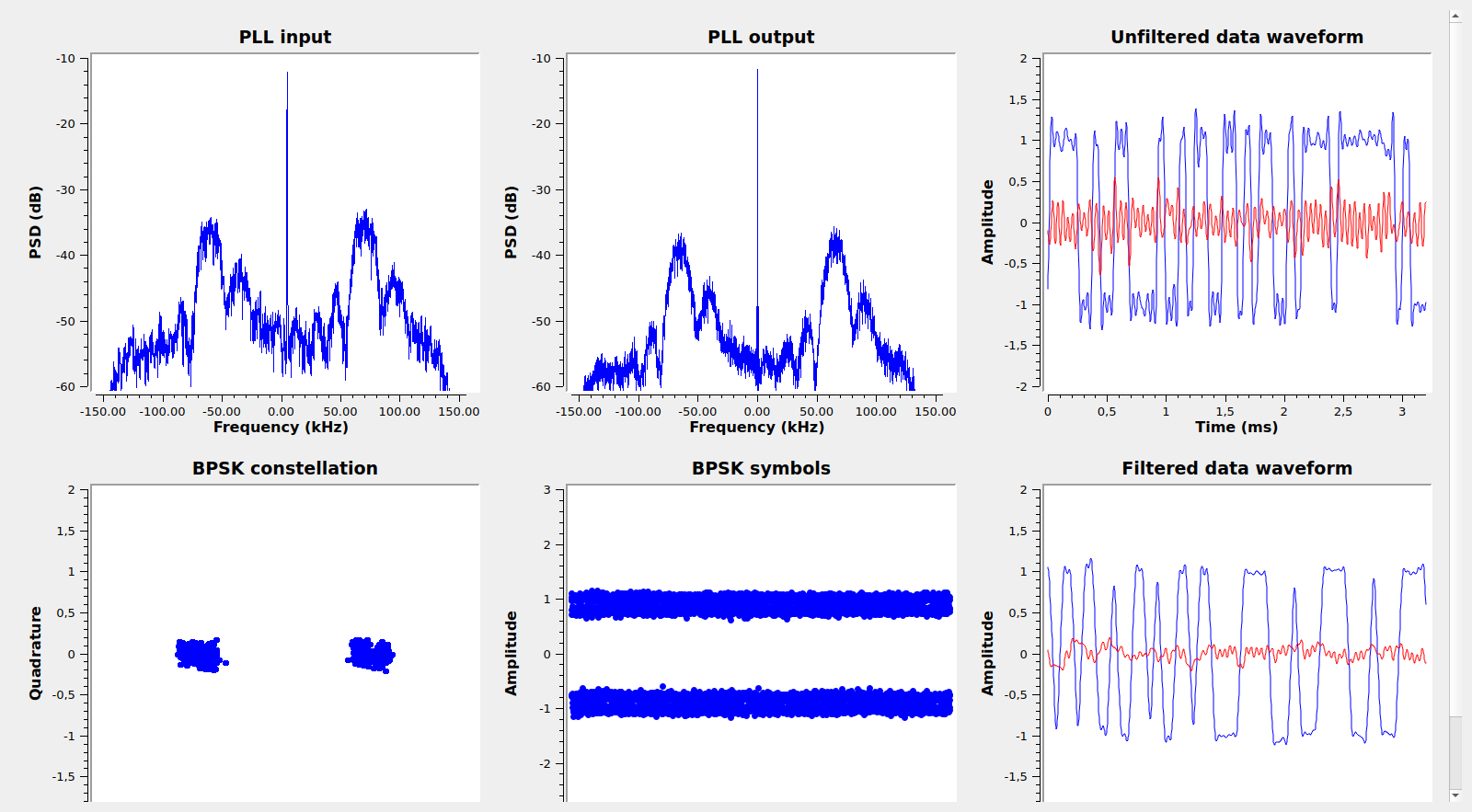
The figure below shows the GNU Radio decoder running on a recording made at Bochum earlier today. It displays the spectrum of signal, both before and after locking the residual carrier, so that signal quality and PLL lock can be assessed. It also shows the constellation symbols and filtered and unfiltered waveforms corresponding to the BPSK data subcarrier.

The figure below shows the full spectrum of the telemetry signal. This is taken from a recording made by AMSAT-DL with the 20m dish at Bochum observatory on 2020-07-26 07:47:20 UTC, after the spacecraft switched to its high gain antenna on 2020-07-26 00:30 UTC.
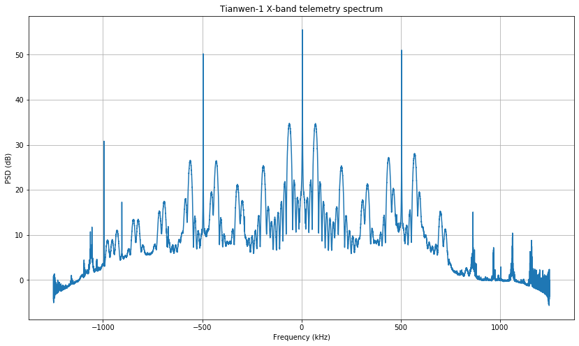
A thing to note here is that the data sidelobes only have odd harmonics. This means that the subcarrier is a square wave, because phase modulation with a sine wave produces both even and odd harmonics, while phase modulation with a square wave produces only odd harmonics.
Besides the central residual carrier and the data subcarriers at +/- 65.536 kHz, there are two CW subcarriers at +/- 500 kHz. Most likely these are used for ranging, as delta-DOR tones. Since everything is phase-modulated onto the same carrier, and phase modulation is inherently non-linear, everything intermodulates. Thus, we see the data subcarriers intermodulating with the CW subcarriers, and producing sidelobes at +/- 65.536 kHz from these (and also some odd harmonics).
In fact, with strong SNR, it is possible to lock the decoder onto one of the CW subcarriers and produce valid data from the intermodulation sidelobes. The figure below shows the decoder happily doing just that. Note the asymmetry of the spectrum, which is caused by the fact that the 7th and 9th harmonic of the data subcarrier also lie around here. This is more of a curiosity than something with a practical application.
The transmitter is also capable of high speed data. In fact, Ferruccio IW1DTU caught the probe transmitting what seemed like BPSK/NRZ (or maybe PCM/PM/NRZ with a weak residual carrier) on 2020-07-26 23:19 UTC. Unfortunately there is no recording of that event and we haven’t seen the spacecraft transmitting high speed data again.
Interestingly, Tianwen-1 has made an image of the Earth and Moon, and this appeared yesterday in the media. That high speed data event might have been used to transmit the image. The astute reader might be able to work out when the image was taken from the angular size of the Earth and the Moon, their angular separation in this image, and Tianwen-1’s trajectory. The media says that it was taken at 1.2 million km away, so according to my ephemerides table that would be around 2020-07-26 21:20 UTC.
The figure below shows the full decoder flowgraph, which can be downloaded here. Click on the figure to view it in full size.
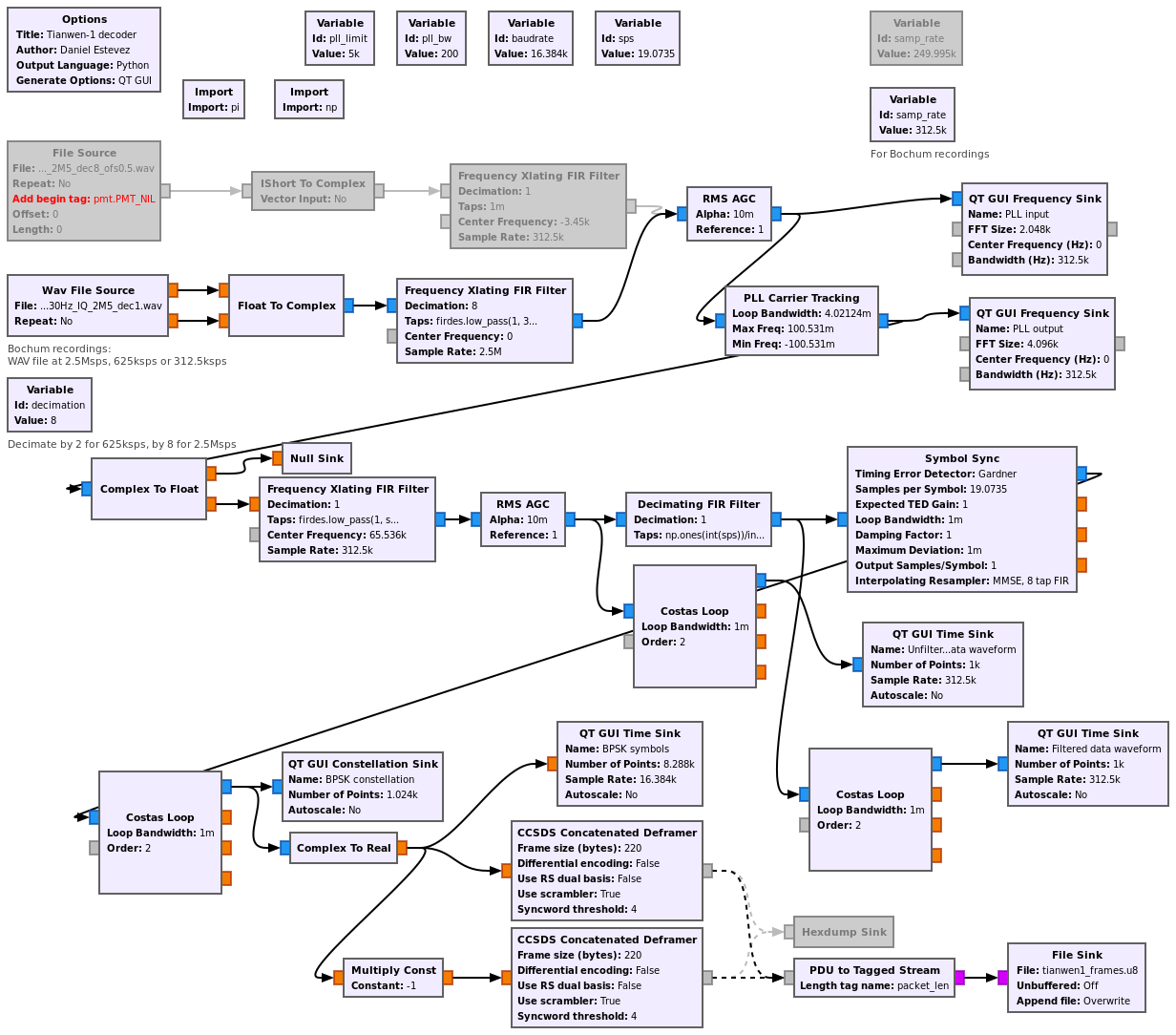
The decoder can work with the recordings from Paul Marsh M0EYT, which use a sample rate of 249.995ksps, and with those made at Bochum, which use 2.5Msps, 625ksps or 312.5ksps (in all cases we decimate first to 312.5ksps). It can easily be adapted to use other sample rates.
To demodulate the signal we first use a PLL to lock the residual carrier. I’m using a loop bandwidth of 200Hz, and certainly it could be made smaller, but so far the SNR is strong enough for this high bandwidth and I don’t want to have problems with carrier dynamics due to the receiver clock or uncorrected Doppler.
After carrier recovery, we use the following method to demodulate the data subcarrier. First we take the imaginary part of the signal, since that is where most of the phase modulation power is. This has the effect of adding up the power in the two data sidebands to form a single BPSK signal at the subcarrier frequency.
An alternative idea to taking the imaginary part is to perform phase demodulation and use the complex argument instead, to try to use all the modulation power. I haven’t put much mathematical thought into this, but from some small experiments this works worse, at least for this phase deviation. Additionally, since phase demodulation is non-linear, the data subcarriers need to be bandpass filtered before taking the complex argument.
In any case, we end up with a real signal with a BPSK signal at the subcarrier frequency. We demodulate this as usual. We move it to baseband, obtaining an IQ signal again, then perform filtering (here I’m using a square-wave non-matched filter), clock recovery (done here with Gardner’s TED) and carrier recovery with a Costas loop. The Costas loop is actually locking to the subcarrier frequency, so its bandwidth can be kept rather small.
Note that the subcarrier frequency is actually four times the baudrate. This means that there are exactly four subcarrier cycles per symbol. This integer relationship is not a coincidence. Most likely the subcarrier and symbol clock are coherent, in the sense that if the symbols start at instants \(t = nT\) for \(n \in \mathbb{Z}\), then the subcarrier is \(\operatorname{sign}(\sin(8\pi t/T + \varphi))\) (or \(\sin ( 8 \pi t / T + \varphi ) \) for a sine wave subcarrier), where \(\varphi\) is typically chosen to be zero but can also be \(\pi/2\). This is the same as the BOC sine and BOC cosine waveforms in GNSS.
In practice, this means that the subcarrier and symbol clock are one and the same and could be recovered using the same loop, whose error can be fed from a weighted average of the TED and the Costas loop discriminator. I haven’t attempted to implement this technique.
After demodulation we perform frame synchronization and FEC decoding. The frames are CCSDS concatenated frames with a size of 220 bytes, as described in the TM Synchronization and Coding Blue Book. As pointed out by r00t, the conventional rather than the dual basis is used for the Reed-Solomon code, so this is somewhat non-compliant with CCSDS.
Though yesterday I commented about the fact that Beijing time is often used with Chinese spacecrafts, here I can’t offer much wisdom about the common use of Reed-Solomon by the Chinese. I can comment that the Amateur satellites made at Harbin Institute of Technology LilacSat-2 and BY70-1 use the conventional basis, and that the lunar satellites Longjiang-1/2, also made by Harbin, used the conventional basis for telecommand (Turbo codes were used for the downlink). In contrast, KS-1Q used the dual basis. Warmonkey, who worked in KS-1Q, made a very interesting comment back in the day about the computational advantage of implementing the conventional basis on a CPU and the dual basis on an FPGA.
The CCSDS concatenated deframer from gr-satellites is used to perform Viterbi decoding of the convolutional code, detect the 32 bit ASM and perform descrambling and Reed-Solomon decoding. We have a 180º phase ambiguity on the BPSK symbols. Even though the original PCM/PSK/PM signal doesn’t have any phase ambiguity, we’ve lost this with our Costas loop based subcarrier recovery. Another way of looking at this is that we haven’t used anywhere (and in fact we don’t know) the value of \(\varphi\) introduced above. Adding \(\pi\) to \(\varphi\) changes the phase of the BPSK symbols by 180º.
Therefore, two deframers are run in parallel: one on the stream of symbols, another on the stream of inverted symbols. Since there is also an ambiguity when pairing symbols at the input of the Viterbi decoder (this is handled inside the CCSDS concatenated deframer from gr-satellites), we have in fact four Viterbi decoders running in parallel.
After Reed-Solomon decoding is done, the 220 byte frames are stored into a file. This file can be read later with extract_state_vectors.py to print out the orbit state vectors that are sent in the telemetry.
I’ll close with two additional remarks. First, an anecdote and warning. When attempting to decode the signal, at first I assumed that the frame size was 223 bytes. This is a common frame size because it is the maximum allowed by a (255, 223) Reed-Solomon codeword. Due to the cyclic properties of Reed-Solomon codes, if we make a small mistake in the size, the decoder will still work.
For example, in this case the decoder takes three additional bytes of garbage (actually the first 3 bytes of the ASM of the next frame) after the real codeword, and provided there are not many byte errors in the real codeword it will just correct these three garbage bytes into the appropriate parity check bytes just as if they were byte errors (recall that such a Reed-Solomon code can correct up to 16 byte errors). The frame will be cropped to 223 bytes, leaving the first 3 parity check bytes at the end. These 3 bytes seem random, as if they were a CRC (and in fact I must recognize that I spent some time trying to see if they were a CRC-24).
So the lesson is to be careful about Reed-Solomon frame sizes and always check the number of byte errors corrected by the Reed-Solomon decoder. If this is never zero, suspect that maybe the frame size is wrong. Often there is no padding between frames, so the correct frame size can be observed by noting the distance between consecutive ASMs.
The final remark is about why a frame size of 220 bytes instead of 223 bytes. Well, there is a good reason. If we add to this the 32 Reed-Solomon parity check bytes and the 4 bytes of the ASM we end up with 256 bytes, which is a power of two, just like the baudrate. This means that, taking into account the convolutional encoding, a frame takes exactly 0.25 seconds to transmit. This is good because it allows a regular frame structure. For instance, the orbit state vectors can be sent every 32 seconds by sending one every 128 frames.
Fantastic work, as usual. We gotta meet one of these years.
I have made a recording of Tianwen-1 X-band signal today with my 4.5 m dish. You can download the file and some HDSDR screenshots here:
http://gs1.to.ee/public_to117/Obs/Viljo/dsn/tianwen/
Recording format is raw 32 bit float, 391 ks/s
Hi Viljo, thank you for sharing this. This can serve for other people to test the decoder. I tested both of the recordings and they run well. Only the loop bandwidth for the Symbol Sync and Costas loop need to be increased.
Hi Daniel,
I have added more recordings on the server, now there are 312.5 ks/s and 625 ks/s recordings in separate folders. They are now in float wav format. I’m also trying to get the gnuradio decoder working, but unfortunately I see no output from the CCSDS deframer block. All plots from the decoder look very similar to the ones shown in your blog page.
I get “correlate_access_code_tag_bbx – writing tag at sample yyy” debug messages randomly. But when I change access code thresholds from 4 to 0 I get no tag write messages. Symbol sync block output looks fine.
GNURadio version is 3.8.1.0. python 3.8.2, gr-satellites-3.2.0, OS Ubuntu 20.04.1
73,
Viljo ES5PC
Hi Viljo,
I have just tested the decoder with one of the 312.5ks/s recordings and it works well for me. The exact decoder I’ve used is here, so please make sure to use this to see if it is a problem with your system. I used the file HDSDR_20200807_194352Z_8430927kHz_RF_flt32_001.raw to test this.
Hi Daniel,
Thank you for the help!
Tested it, but still seems to have the same problem. Screenshots are here:
http://gs1.to.ee/public_to117/Obs/Viljo/dsn/tianwen/312.5ks/Tianwen_dec_008.jpg
http://gs1.to.ee/public_to117/Obs/Viljo/dsn/tianwen/312.5ks/Tianwen_dec_009.jpg
I have also activated the hexdump block, but there seem to be no output from it.
73,
Viljo
Two things you can do: activate the verbose reporting of the Reed-Solomon decoder by using “–verbose_rs” as the Command line option parameter of the CCSDS deframer block.
Maybe your problem is this problem with the Viterbi decoder, so please run volk_profile just to be sure.
After volk_profile it works fine. Thank you very much for help!
73,
Viljo
Hi,
I have uploaded more RF files and decoded frames data on the server in 312.5ks and 650ks folders.Decoder works now fine with both sample rates. I can also try to set up real time decoding with USRP source instead of file source on gnuradio.
73,
Viljo ES5PC
Hi.
I want to simulate PCM/BPSK/PM in matlab software, but I cant do this correctly. First Bpsk modulation and then PM, But i Don’t see residual carrier. why? please help me.
Hi Alex,
Without more information about what you’re doing I can just say that you must be doing something wrong. If you take any real signal with amplitude not larger than one and phase modulate it with a deviation smaller than pi/2, the resulting signal will have a residual carrier. The reason is that the real part of such signal is positive, so the signal has non-zero average.
Do You do phase modulation using which formula? I use from the equation mententioned in: https://deepspace.jpl.nasa.gov/files/phase1.pdf
Phase modulation is phase modulation, regardless of which formula you use. However, just for the sake of clarity, I was talking about the complex baseband representation, so the formula would be exp(i*d*x(t)) where d is the deviation and x(t) is the real modulating signal.
Hi Daniel,
I work with pcm/psk/pm modulation and I created more or less the same RX chain as you have. However, it seems to me that such a chain is not optimal in terms of reception quality. The bit error rate should be the same as with BPSK modulation: BER = 0.5*erfc(sqrt(Eb/N0)). With the mentioned chain, I have losses of about 3 dB compared to the reference formula. Specifically, the BER for 9.6 dB should be 1e-5. The current chain achieves this on about 12.6 dB. What are your thoughts and experience about this?
It partly depends on the subcarrier used for telemetry. For a square wave subcarrier, since this receiver is using a sine subcarrier, there are some associated losses. These are -0.91 dB, which is the power on the fundamental of a square wave, as described in https://destevez.net/2022/12/a-note-about-non-matched-pulse-filtering/
For a sine subcarrier, only the fundamental can be used. Bessel functions can be used to compute how much power phase modulation puts on the fundamental, depending on the deviation.
I’m aware that, let’s say, using different subcarriers on TX and RX would produce some loss, but the mentioned 3 dB loss happens with a sine subcarrier.
The signal is indeed downconverted with the fundamental (subcarrier) frequency, after taking the imaginary part, using the Xlating FIR filter. Therefore, with your very same chain, I get 3 dB of loss (target is the same as for BPSK: BER=1e-5 for EbN0 9.6 dB is expected) and I don’t know where it comes from.
If we take the imaginary part from the phase modulated signal, the fundamental frequency within it holds 93% of the power and the rest of the harmonics carry 7%. I suspect that it produces the mentioned loss.
Thank you for help and fast response.