Decoding Voyager 1

Today is the 44th anniversary of the launch of Voyager 1, so I want to celebrate by showing how to decode the Voyager 1 telemetry signal using GNU Radio and some Python. I will use a recording that was done back in 30 December 2015 with the Green Bank Telescope in the context of the Breakthrough Listen project. Most of the data from this project is open data and can be accessed through this portal.

In contrast to other posts about deep space probes in this blog, which are of a very specialized nature, I will try to keep this post accessible to a wider audience by giving more details about the basics. Those interested in learning further can refer to the workshop “Decoding Interplanetary Spacecraft” that I gave in GRCon 2020, and also take a look at other posts in this blog.

Handling the raw recording

The direct link to the 16 GB recording that I will use is this one. This recording is in GUPPI fomat, which is a format that stores the raw IQ output (voltage mode) from a filter bank. This kind of file is often processed to transform it to make it easier to use for a particular application and reduce the data size. For instance, in this Jupyter notebook from Breakthrough Listen, a file in filterbank format produced from this data is used to plot the signal spectrum. The filterbank format is essentially some kind of high-resolution waterfall data (power versus time-frequency), and it is often used in SETI (this recording of Voyager 1 was made to test SETI algorithms). Here we need to use the raw IQ data in the GUPPI file to process the digital modulation. I also used this GUPPI file in a post from a few years ago about the Voyager 1 polarization.

The data in the GUPPI file is divided in 64 frequency channels, each of them having a bandwidth of 2.9296875 MHz, which gives a total observing bandwidth of 187.5 MHz (the division by 64 explains the rather peculiar sample rate of each individual channel). The centre frequency of the observation is 8493.75 MHz, and the Voyager-1 signal can be found at 8420.216454 MHz.

In comparison to the large bandwidth observed in this recording, the Voyager-1 signal is tiny. It fits in less than 100 kHz. Luckily, it is contained entirely in one of the 64 channels of the GUPPI file, which simplifies the processing. We can use this single channel and throw away the rest, instead of having to glue two adjacent channels to produce a single stream of IQ data.

The IQ data in each channel is stored as 8-bit integers. The only quirk is that the frequency axis is inverted in each channel, so the sign of Q needs to be flipped to correct this (another possibility is to swap I and Q). In radio astronomy it is very common to quantize with a low number of bits, such as 4 bits or 2 bits, since the signals typically have low SNR.

The file contains the two circular polarization channels: LHCP and RHCP. Since the Voyager-1 signal is LHCP, we will only use that channel. The recording is rather short. Its duration is only 22.57 seconds.

All these technical details about the file format are contained in the GUPPI file itself. This file format has a header with metadata in ASCII, then a block with binary data, then another ASCII header followed by more binary data, and so on. The first header contains the following:

BACKEND = 'GUPPI '
TELESCOP= 'GBT '
OBSERVER= 'Dave MacMahon'
PROJID = 'AGBT16A_999_07'
FRONTEND= 'Rcvr8_10'
NRCVR = 2
FD_POLN = 'CIRC '
OBSFREQ = 8493.75
SRC_NAME= 'VOYAGER1'
TRK_MODE= 'TRACK '
RA_STR = '17:11:58.7280'
RA = 257.9947
DEC_STR = '+11:56:57.4800'
DEC = 11.9493
LST = 79318
AZ = 268.5982
ZA = 68.8151
BMAJ = 0.02453834653321856
BMIN = 0.02453834653321856
DAQPULSE= 'Wed Dec 30 15:45:27 2015'
DAQSTATE= 'running '
NBITS = 8
OFFSET0 = 0.0
OFFSET1 = 0.0
OFFSET2 = 0.0
OFFSET3 = 0.0
BANKNAM = 'BANKD '
TFOLD = 0
DS_FREQ = 1
DS_TIME = 1
FFTLEN = 32768
CHAN_BW = 2.9296875
NBIN = 256
OBSNCHAN= 64
SCALE0 = 1.0
SCALE1 = 1.0
DATAHOST= '10.17.0.142'
SCALE3 = 1.0
NPOL = 4
POL_TYPE= 'AABBCRCI'
BANKNUM = 3
DATAPORT= 60000
ONLY_I = 0
CAL_DCYC= 0.5
DIRECTIO= 0
BLOCSIZE= 132251648
ACC_LEN = 1
CAL_MODE= 'OFF '
OVERLAP = 512
OBS_MODE= 'RAW '
CAL_FREQ= 'unspecified'
DATADIR = '/datax/dibas'
PFB_OVER= 12
SCANLEN = 300.0
PARFILE = '/opt/dibas/etc/config/example.par'
OBSBW = 187.5
SCALE2 = 1.0
BINDHOST= 'eth4 '
PKTFMT = '1SFA '
TBIN = 3.41333333333E-07
BASE_BW = 1450.0
CHAN_DM = 0.0
SCANNUM = 4
SCAN = 4
NETSTAT = 'receiving'
DISKSTAT= 'waiting '
PKTIDX = 0
DROPAVG = 4.18843e-07
DROPTOT = 0.536095
DROPBLK = 0
STT_IMJD= 57386
STT_SMJD= 74728
STTVALID= 1
NETBUFST= '1/24 '
SCANREM = 300.0
STT_OFFS= 0
PKTSIZE = 8192
NPKT = 16143
NDROP = 0
END

To process this file in GNU Radio, I use an Embedded Python Block that reads data from one of the channels of the file. The code in this block is based on the Python code I used in my older post, which in turn is based on code from blimpy, which is a Python tool used by Breakthrough Listen to manipulate file formats. I originally made this Embedded Python Block for a session with the Berkeley SETI Research Center REU summer students this year. In that session I used this block to show the students how to use GNU Radio to display the spectrum of the signal in different ways.

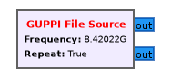
This GUPPI File Source block is shown below. It is something very crude, as it has almost all the parameters hardcoded, including the path to the GUPPI file. It has a “frequency” parameter that it is used to select the frequency channel that the file source will use. It will only use the channel that contains that particular frequency. Its two output ports give each of the two polarization channels as complex floating point data.

This GUPPI File Source block can be used to prepare a reduced file that only contains the LHCP polarization of the frequency channel in which the Voyager 1 signal is present. The flowgraph shown below performs the reduction. Note that neither the GUPPI File Source nor the Complex To IChar are changing the scale of the samples, so we end up with the same 8-bit samples that were present in the GUPPI file.

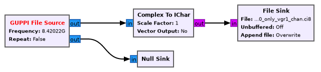
The advantage of performing this reduction is that the resulting file has a size of only 127 MB. This reduced file can be downloaded here, and is the file that will be used in the rest of this post.

A brief look at the modulation

Even with Green Bank’s 100 metre telescope, the Voyager 1 signal is weak enough that it is difficult to detect in the 2.9296875 MHz channel from the GUPPI file unless a large FFT size and long integrations are used. The material from my Breakthrough Listen REU session shows how to do so.

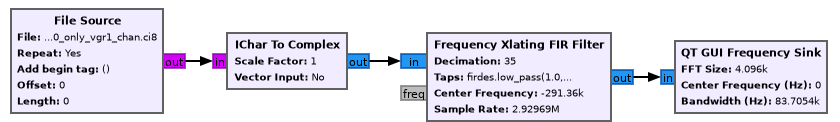
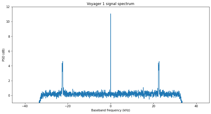
If we know exactly at which frequency the Voyager 1 signal is located, it is easier to use the Frequency Xlating FIR Filter block to move the signal to baseband and decimate by a factor of 35, giving a sample rate of ~83.7 kHz. This allows us to see the signal more easily with a modest FFT size of 4096 points. The GNU Radio flowgraph used to plot the spectrum with this technique is shown here.

In the resulting plot we can see the residual carrier of the signal as a strong and very thin peak in the middle and the data subcarriers as thin humps at ±22.5 kHz from the carrier.

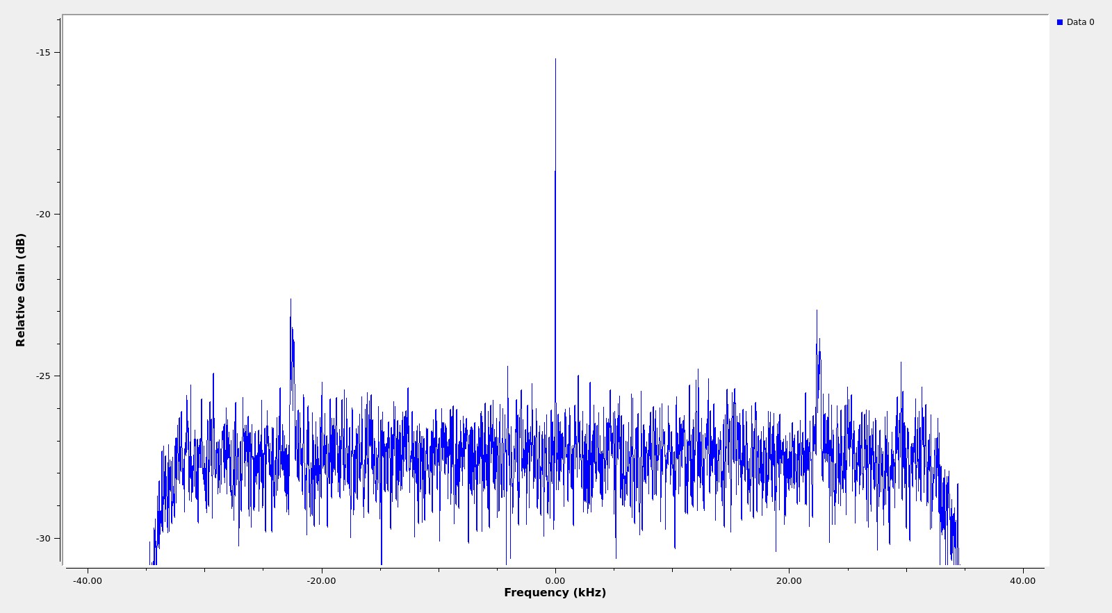
This kind of modulation is used very frequently to transmit low rate telemetry from deep space probes. Its technical name is PCM/PSK/PM (see this document) and it is a residual carrier phase modulation. People familiar with my posts about deep space probes might recognise that Tianwen-1, Chang’e 5, and many others I haven’t studied in detail also use this kind of modulation.

A substantial amount of the transmitted power is spent in the carrier, which is the very thin, unmodulated line we see in the middle. This relatively strong residual carrier allows the people on ground to detect the signal even if there are problems that cause it to be much weaker than expected, to have a reference to track the phase of the signal (which is important at these microwave frequencies), and to measure Doppler very accurately, which is used to help determine the trajectory of the spacecraft.

The rest of the transmitted power is spent in sending the data, which is modulated into subcarriers at both sides of the carrier (in this case at ±22.5 kHz). The data is PSK-modulated onto these subcarriers, so by looking at the width of the subcarriers we can get an approximate idea of the data rate. In this case the subcarriers are thin: around 300 Hz wide or so, since the data rate is not very high. Since Voyager 1 is extremely far from Earth, it typically uses rather low data rates so that it can be decoded with one 70 metre or several 34 metre antennas of the NASA DSN.

The separation between the data subcarriers and the carrier is given by the subcarrier frequency (22.5 kHz here). The purpose of separating the subcarriers is to prevent the data modulation from interfering with the phase tracking of the carrier. Often, a larger separation than strictly necessary is used. The gap between the data subcarriers and the carrier is sometimes used to retransmit sequential ranging tones or telecommand feed-through (which consists in relaying the telecommand signal back to Earth so that people can check that the spacecraft receives it with enough quality).

The figure below shows a better view of the spectrum of the Voyager 1 signal. It has been obtained by using an FFT size of 4096 points (~20 Hz resolution) and averaging across all the recording length.

Carrier tracking

The first step in processing this signal is to track the residual carrier, in order to estimate and correct for the Doppler and phase offset of the signal. This is done with a PLL. The figure below shows the part of the GNU Radio flowgraph corresponding to the PLL. Since the PLL expects a signal of amplitude one, we use the RMS AGC block from gr-satellites to normalize the signal amplitude.

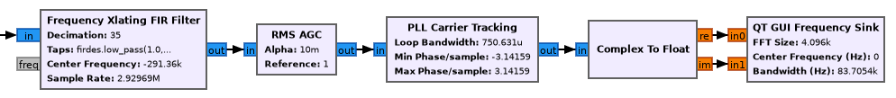
A small loop bandwidth should be used for best results (less tracking jitter) in the PLL. If the bandwidth is set too low, the loop will not lock, though. Here a bandwidth of 10 Hz is used. Note that the units of the loop bandwidth parameter in the PLL Carrier Tracking block are radians per sample rather than Hz.

At the output of the PLL, the real part of the signal contains the suppressed carrier and the imaginary part contains most of the power of the data sidebands, due to how phase modulation works. This can be seen in the figure below, which shows the real part in blue and the imaginary part in red.

Data demodulation

Usually, the data would be demodulated by synchronizing to the symbol clock with the Symbol Sync block and tracking the subcarrier with a Costas Loop. However, these loops take some time to lock, specially when low bandwidths are used, which is important to deal with weaker signals. Since the recording is only 22.57 seconds long, we will do an open loop demodulation in Python adjusting by hand some of the parameters. This will allow us to demodulate all the data with good performance.

First we use GNU Radio to move the data sideband from 22.5 kHz down to 0 Hz. Note that now the signal is real, being the imaginary part of the output of the PLL, so the spectrum is symmetric. By performing downconversion we obtain a complex IQ signal again in which the data modulation looks like BPSK. Since the data sideband is narrow, we can low pass filter and decimate. All these steps can be accomplished at once with the Frequency Xlating FIR Filter block in GNU Radio. The flowgraph to do so is shown below. We take the imaginary part of the output of the PLL, and decimate by 50 while filtering and downconverting the data subcarrier. The output is saved to a file which is later processed in Python.

We load up the file in Python and plot the spectrum using NumPy and Matplotlib (the code is provided in a Jupyter notebook at the end of the post). We get the figure below. At ±350 Hz we have the cut-off of the filter used in the Frequency Xlating FIR filter. We could have used a higher cut-off frequency if we just wanted to prevent aliasing when decimating, but by adjusting the cut-off to be just slightly larger than the signal bandwidth, we discard a good portion of the noise.

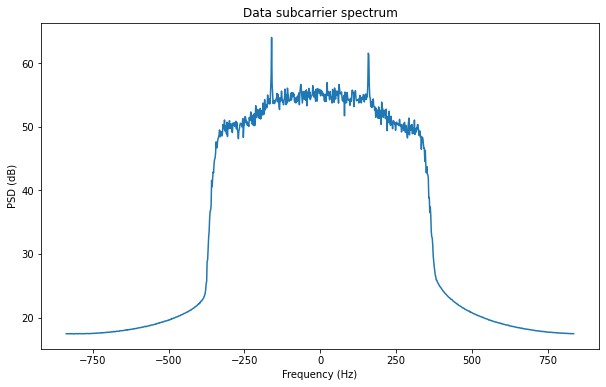
The data signal is actually the hump of a few dB between -240 Hz and 240 Hz. There are two tones at the edges of the signal. The reason for this will be explained later.

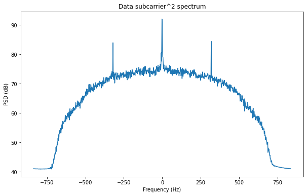
The next step is to remove the residual subcarrier frequency and phase. We have already subtracted the nominal 22.5 kHz subcarrier, but there is still a small residual frequency due to Doppler and different clocks at the transmitter and receiver. This residual frequency is present as the suppressed carrier of the BPSK signal we are dealing with. The trick to recover the suppressed carrier is to square the signal (raise it to the power two). This reveals a tone whose frequency is twice the suppressed carrier frequency, basically because it removes the BPSK modulation. The reason behind it is that 1²=(-1)²=1. The figure below shows the resulting spectrum. We see that a strong tone has appeared near 0 Hz.

Now we can low pass filter the central tone to remove much of the noise and measure its phase. Dividing the phase by two (after unwrapping) we obtain the phase of the residual subcarrier. We can use it to remove the residual subcarrier. Then we should should obtain the BPSK signal in the real part, together with noise. In the imaginary part we should get only noise. This is shown in the figure below.

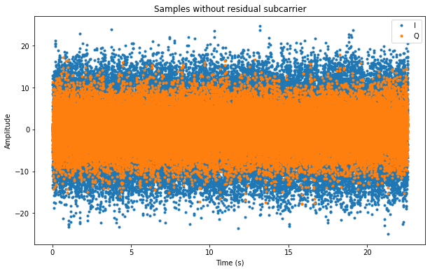
The real part (or I, for in-phase) is shown in blue, while the imaginary part (or Q, for quadrature) is shown in orange. The amplitude of I is somewhat larger than the amplitude of Q due to the presence of the BPSK signal in the I component. The SNR of the signal is rather low, but if it was higher, the amplitude difference between I and Q would be larger.

The plot above indicates that our removal of the subcarrier has been successful, since otherwise the phase of the BPSK signal would rotate and we would see the same amplitude in I and Q. The next step is to recover the symbol clock and demodulate the symbols. For that, we first need to know the symbol rate or baudrate.

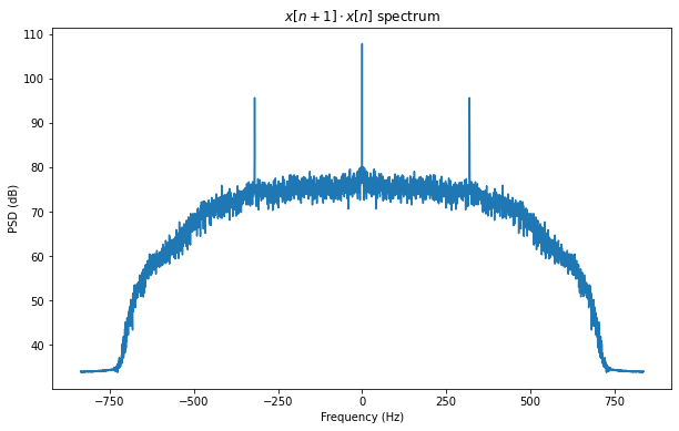
The trick to find the baudrate is to take the signal (here we can take the real part after removing the subcarrier) and multiply it against the same signal delayed one sample. Then we plot the spectrum of the result. What we see is quite similar to the spectrum of the square of the signal we did before. Here the presence of tones at ±320 Hz indicates that the symbol rate is 320 baud.

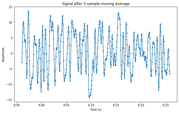
With this knowledge, we can align the sample clock by hand. At the sample rate we are using there are approximately 5.231 samples per symbol. First we run the signal through a moving average of 5 samples in order to add up most of the power in each symbol. We see the result in the figure below, where individual samples have been marked with a dot. Even though the signal is noisy, we can recognise the bits as the positive (bit value 1) and negative (bit value 0) peaks.

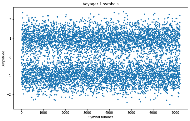
Our goal is to take one out of every 5.231 samples in such a way that we are aligned to the peaks of the signal, which correspond to the optimal sampling instants. The thing we can vary is to slide our choice of sampling instants forwards or backwards in time. This corresponds to trying to find the phase of the symbol clock. We also account for a small deviation from the nominal symbol rate of 320 baud. After fiddling for a little with the parameters, we obtain the figure below. We have also normalized the signal to unit amplitude. We can now see that most of the values cluster around +1 or -1. There are some values around 0 which will give symbol errors, but all in all the signal quality is not so bad.

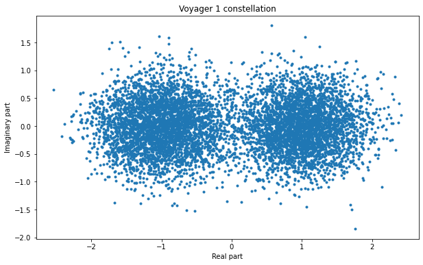
We can also plot the constellation, which shows all the symbols in the complex plane (remember that the BPSK signal was present in the real part, but we also had the imaginary part, which only contained noise). We see two areas where the symbols concentrate, corresponding to the bits 1 and 0.

This finishes the data demodulation.

Viterbi decoding

The Voyager probes use the typical k=7, r=1/2 convolutional code as a forward error correction method. In fact they were among the first spacecraft to use this code. A Viterbi decoder can be used to correct for bit errors and obtain the original message.

The convolutional code produces a pair of bits for each input bit. These two bits are transmitted sequentially. At the receiver, we need to pair the two bits again. There are two possible ways to do this, given by the two possible arrangements of drawing lines between symbols in a stream in order to divide them up in pairs.

There are different techniques to decide which is the correct pairing. A simple but effective way to do this consists in running the Viterbi decoder separately for each of the two possibilities, encode back with the convolutional encoder each of the two outputs, and compare them with the received data to count the number of bit errors. The correct choice will give a relatively low number of bit errors.

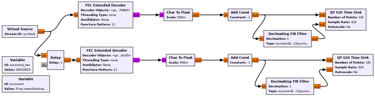
We use GNU Radio to do Viterbi decoding and convolutional encoding, using the flowgraph shown below.

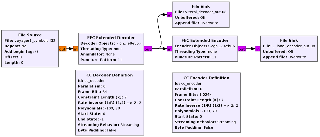
The data is read from a file that was produced with the Jupyter notebook. Then both the decoded output and the re-encoded output are written to files. For the input of the Viterbi decoder we are using soft symbols, which preserve the amplitude data and give much better error correction performance than hard symbols (which are just 1’s and 0’s).

In this case, to pair the received symbols correctly we need to throw away the first symbol, so that the symbols that get paired are the second and third together, fourth and fifth, etc. It might have happened that the correct pairing was the first and second together, third and fourth, etc. In that case we wouldn’t throw away the first symbol.

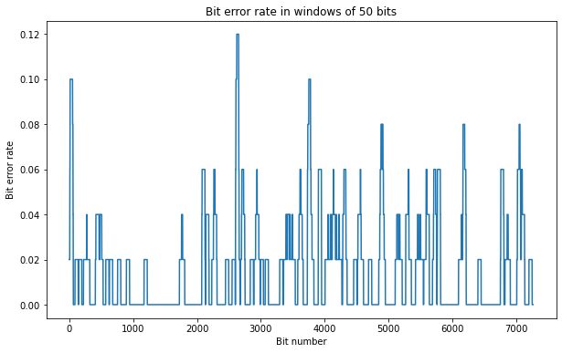
In the Jupyter notebook we can compute the average bit error rate and see that it’s only 1.6%, which is quite good. Presumably all these bit errors would be corrected by the Viterbi decoder. The figure below shows the bit error rate measured in a moving window of 50 bits. We see that occasionally around 5 out of 50 bit are wrong, but we also have some relatively long periods without any bit errors.

Something worth mentioning is that Voyager 1 uses the legacy NASA-DSN convention for the convolutional code instead of the more modern CCSDS convention. The difference between these two conventions is just the order in which the two bits in each encoded pair are sent, as described in Figure 3 of this document.

Finding the ASM

The next step in decoding is to find the Attached Synchronization Marker (ASM), which is a fixed sequence (often 32 bits long) that marks the beginning of each frame. If we know which ASM is used, we can simply correlate the decoded bits with the ASM to find in which places the ASM appears (even if there are some uncorrected bit errors). If we don’t know the ASM, sometimes it is possible to find it by correlating the decoded bits with themselves and finding which parts of the data repeat.

The CCSDS standards recommend the use of the ASM 0x1ACFFC1D for convolutionally encoded data (and for other types of data as well). See Section 9 in the TM Synchronization and Channel Coding Blue Book. This choice of ASM is followed in the present day by many missions. However, it turns out that Voyager 1 uses a different ASM, since it probably predates the standardization of 0x1ACFFC1D.

I have to thank Richard Stephenson, from Canberra DSN, for telling me that the ASM used by the Voyager probes is 0x03915ED3. It is very difficult to find this data on the internet, since there doesn’t seem to be detailed documentation for how the telemetry transmission of Voyager works. Nevertheless, there is a very interesting report from DESCANSO about Voyager telecommuncations. It also appears as a chapter in this book. However, it focuses more on the RF side of things and does not give all the details about the digital communications aspects.

Here we have some difficulties, because the frame length used by Voyager 1 for transmission at 320 baud is 7680 bits. Taking into account that due to convolutional encoding the net data rate is 160 bps, a frame takes 48 seconds to transmit. Since our recording is only 22.57 seconds long, we don’t even have a complete frame inside the recording. However, it turns out we’re lucky and we have the beginning of a frame, including the ASM.

The figure below shows the results of the correlation of the bits we have decoded with the ASM 0x03915ED3. If the ASM is present somewhere in the bits, we expect to see a peak with a value close to 32 or -32 at the location corresponding to where the ASM appears in the bit sequence. The reason why the value could be positive or negative is that there is a 180º phase ambiguity in the subcarrier recovery we did, so we may be looking at the original bit sequence or at the inverted bit sequence (where each 1 has been replaced by a 0 and vice-versa). By detecting whether we see the normal ASM or its inversion, we can detect and correct this ambiguity. The reason why the correlation value could be different from 32 (corresponding to 32 bits matched with the ASM) is that in principle there could still be a few uncorrected bit errors after the Viterbi decoder (though in this case probably all the bit errors were successfully corrected).

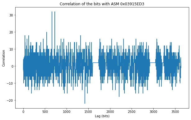
We see that the ASM appears two times near the beginning of the data. These two appearances are 64 bits apart, which means that we have the 32-bit ASM, then 32 bits with some other data, and then once again the 32-bit ASM. Then the frame starts, and its end is beyond the end of the recording. I don’t know why the ASM appears twice.

A look at the data bits

Now that we know the location of the ASM, we can align ourselves to the start of the frame and study the data bits. The figure below shows the bits laid in rows of 64 bits. The choice of 64 bits is convenient because it lays things in a roughly square image, which sometimes makes patterns easier to see, and because this puts the two ASMs in consecutive rows.

I have aligned things so that the ASMs are at the beginning of a row. The ASMs are highlighted in dark purple (0’s) and yellow (1’s). The normal data is shown in blue (0’s) and green (1’s). The teal at the beginning and end corresponds to artificial padding I’ve added to fill in a whole number of rows.

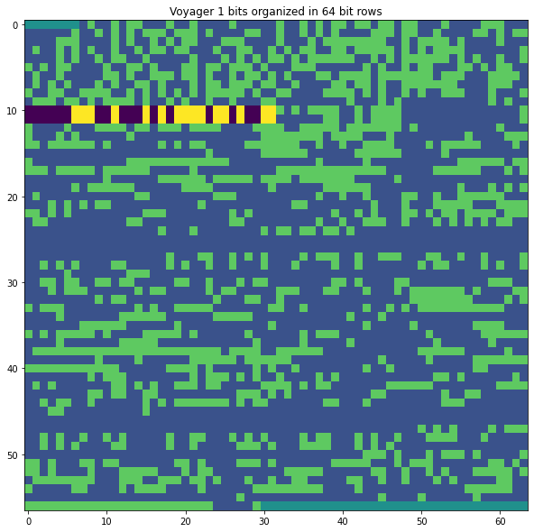
We see that there are two long strings of zeros in the data. The presence of these strings of zeros causes the two tones that we saw at the sides of the data subcarrier (the figure is shown again below for convenience). The reason is that when a string of all zeros (or all ones) is sent through the convolutional encoder, its output will consist of an alternating pattern 01010101… This causes the two tones, since for this pattern the transmitted data looks like a square wave, which has spectral lines.

There is no further error correction (such as Reed-Solomon) used by the Voyager probes, so at this point we have finished decoding the data. We have a small part of the end of one frame, and a good portion of the next one. It is extremely difficult to understand what these contain without a knowledge of how the data is encoded.

If we had a longer recording, we could extract multiple frames and compare them. Sometimes it’s possible to see patterns that help us make some sense of the data. If I manage to get my hands on a longer recording, I will surely take a look and post about it.

More technical data

Once we know that the ASM for the Voyager probes is 0x03915ED3, we can search for this in Google and find very interesting technical information. For instance, Table 1 in page 125 of the “Telemetry Simulation Assembly Implementation in the DSN” progress report gives details for the telemetry of several deep space probes from 1983. This table confirms the ASM for Voyager 2 and shows that Galileo also used the same ASM. Back in 1983, when Voyager 2 was much closer to Earth, it transmitted at 900 bps with a 360 kHz subcarrier.

We also have this file and this file from some obscure URL at NASA. I am not sure what these are, but they seem to contain all the data required by the DSN to track a spacecraft (run a support, as they usually call it). They date from February 2017 and contain some XML, but also some lists in plain text embedded in the XML. At some point in these files we have several TELEMETRY_INFO tables with an exact definition of the telemetry parameters. The relevant entry for the recording we are using is this one:

TELEMETRY_INFO(3)
    SAFE_CFG:  F
    SUB_FREQ_HZ:  22500.0
    SUB_RAMP_FLAG:  F
    SUB_WAVE_FORM:  SQ
    SYM_RATE_HZ:  320.0
    SYM_COHERENT:  F
    SYM_NUM:  1
    SYM_DEN:  1
    INNER_DECD_TYPE:  MCD2
    TRB_RATE_NUM:  1
    TRB_RATE_DEN:  3
    TRB_FRAME_SIZE:  8920
    FS_MODE:  P
    FS_FRM_LEN_PRIMARY:  7680
    FS_BIT_SLIP_WIN:  2
    FS_IL_BET:  1
    FS_OOL_BET:  1
    FS_IL_THRSH:  2
    FS_OOL_THRSH:  2
    FS_PATTERN_LEN:  32
    FS_PATTERN:  03915ED3
    FS_POL:  B
    FA_CRC:  D
    FA_PN:  D
    RS_INTERLEAVE:  0
    RS_FRM_MODE:  D
    RS_HDR_MODE:  D
    DFT_FMT_TBL:  VGR1SFU
    DFT_STRM_MODE:  E
    DFT_CHK_INCLUDED:  E
    DFT_100NSEC_RES:  D
    DFT_ERT_REF:  L
    ALL_FMT_TBL:  VGR1SFU
    ALL_STRM_MODE:  D
    ALL_CHK_INCLUDED:  E
    ALL_100NSEC_RES:  D
    ALL_ERT_REF:  L
    DAS_MODE:  D
    CCSDS_PACKET_TYPE:  0

Other entries give configurations with a different symbol rate: 80 baud, 93.2 baud, 1.2 kbaud, 2.4 kbaud, 2.8 kbaud, 5.6 kbaud, 9.6 kbaud, 14.4 kbaud, and 40 baud (uncoded). These entries show the frame size as FS_FRM_LEN_PRIMARY, which is different for each baudrate, and the subcarrier frequency (SUB_FREQ_HZ) and ASM (FS_PATTERN) , which are the same for all of them. They also show the forward error correction in use. INNER_DECD_TYPE: MCD2 refers to the Viterbi decoder (MCD stands for multi-convolutional decoder).

There are many other interesting details in these files, such as a registry of the system performance including received signal levels and system noise temperature. It is certainly fun to have a thorough look at them.

Software and data

The GUPPI recording used in this post can be downloaded here. it can also be found by searching for target name VOYAGER1 in the Breakthrough Listen open data archive (it has the date 2015-12-30 00:00:00). A much smaller file which only contains the LHCP polarization for the ~3 MHz frequency channel in which the Voyager 1 signal is present can be downloaded here.

The GNU Radio flowgraphs and the Jupyter notebook are in this repository. The following GNU Radio flowgraphs are included.

voyager1_extract.grc, which takes as input the small file that contains only a ~3 MHz channel, locks to the residual carrier with a PLL, and outputs the decimated and filtred data sideband to a file.

voyager1_viterbi.grc, which takes as input the demodulated symbols produced with the Jupyter notebook and runs the Viterbi decoder and convolutional encoder.

voyager1_decoder.grc, which takes as an input the small file that contains only a ~3 MHz channel and performs the complete decoding of the signal, including Viterbi decoding and ASM detection. This is provided for completeness, since due to the short duration of the recording it is better to use an open loop symbol recovery as described in the post to prevent loosing any data due to the acquisition time of the loops.

In this full decoder flowgraph the clock recovery is done by the flowgraph section shown below. The Symbol Sync is used to recover the symbol clock and perform pulse shape filtering. A root-raised cosine pulse shape with the maximum likelyhood time error detector is used in this case, although the choice is not very important. A Costas Loop is used after clock recovery to remove the residual subcarrier.

Viterbi decoding done with the FEC Extended Decoder, using the CC Decoder Definition. The correlation with the ASM is implemented with a Decimating FIR filter and displayed in a QT GUI Time Sink. In order to account for the two possible pairings of received symbols, two copies of the Viterbi decoder are run in parallel. One uses the stream of received symbols, the other uses the same stream but delayed one sample.

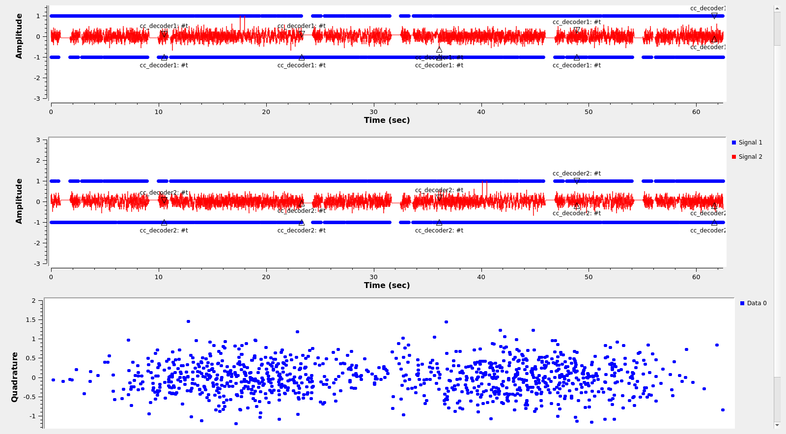
The figure below shows the GUI of the GNU Radio decoder flowgraph running. In the bottom we see the constellation plot. In the top we see the detections of the ASM. Te recording is played endlessly in a loop, so we see detections in both Viterbi decoders, due to bit slip when the recording goes again to the beginning.