More data from Voyager 1

Back in September, I showed how to decode the telemetry signal from Voyager 1 using a recording made with the Green Bank Telescope in 2015 by the Breakthrough Listen project. The recording was only 22.57 seconds long, so it didn’t even contain a complete telemetry frame. To study the contents of the telemetry, more data would be needed. Often we can learn things about the structure of the telemetry frames by comparing several consecutive frames. Fields whose contents don’t change, counters, and other features become apparent.

Some time after writing that post, Steve Croft, from BSRC, pointed me to another set of recordings of Voyager 1 from 16 July 2020 (MJD 59046.8). They were also made by Breakthrough Listen with the Green Bank Telescope, but they are longer. This post is an analysis of this set of recordings.

Recorded data

The recordings follow the usual observing cadence of Breakthrough Listen, described in Section 2.1 in this paper. Six scans of 5 minutes each are done. The primary target (in this case Voyager 1) is observed in three of the scans, called ON scans. In the three other scans, called OFF scans, other targets or the empty sky are observed. The ON and OFF scans alternate, starting with an ON scan. The goal of this schedule is to discard as local interference signals that are present both in an ON and OFF scan.

I think that these recordings have not been published yet in the Breakthrough Listen open data archive. I guess they will be published at some point when the data is curated.

Update 2023-05-19: The recordings are now published here.

The files I used are from compute node BLC23, which processed the data in a 187.5 MHz window around the frequency 8345.21484375 MHz. A total of 24 compute nodes were used in this observation to cover the span between 7501.5 and 11251.5 MHz approximately (a few of the 187.5 MHz windows were duplicated into two nodes).

The files are in GUPPI format, which I described in my previous post. The header of the first file in the dataset is as follows:

 BACKEND = 'GUPPI   '
 DAQCTRL = 'start   '
 TELESCOP= 'GBT     '
 OBSERVER= 'Steve Croft'
 PROJID  = 'AGBT20A_999_53'
 FRONTEND= 'Rcvr8_10'
 NRCVR   =                    2
 FD_POLN = 'CIRC    '
 BMAJ    =  0.02198635849376383
 BMIN    =  0.02198635849376383
 SRC_NAME= 'VOYAGER-1'
 TRK_MODE= 'UNKNOWN '
 RA_STR  = '17:12:40.4400'
 RA      =             258.1685
 DEC_STR = '+12:24:14.7600'
 DEC     =              12.4041
 LST     =                45322
 AZ      =              92.7495
 ZA      =              66.3982
 DAQPULSE= 'Thu Jul 16 18:13:55 2020'
 DAQSTATE= 'record  '
 NBITS   =                    8
 OFFSET0 =                  0.0
 OFFSET1 =                  0.0
 OFFSET2 =                  0.0
 OFFSET3 =                  0.0
 BANKNAM = 'BLP23   '
 TFOLD   =                    0
 DS_FREQ =                    1
 DS_TIME =                    1
 FFTLEN  =                  512
 CHAN_BW =           -2.9296875
 BANDNUM =                    2
 NBIN    =                    0
 OBSNCHAN=                   64
 SCALE0  =                  1.0
 SCALE1  =                  1.0
 DATAHOST= 'blr2-3-10-3.gb.nrao.edu'
 SCALE3  =                  1.0
 NPOL    =                    4
 POL_TYPE= 'AABBCRCI'
 BANKNUM =                    3
 DATAPORT=                60000
 ONLY_I  =                    0
 CAL_DCYC=                  0.5
 DIRECTIO=                    1
 BLOCSIZE=            134217728
 ACC_LEN =                    1
 CAL_MODE= 'OFF     '
 OVERLAP =                    0
 OBS_MODE= 'RAW     '
 CAL_FREQ=                  0.0
 DATADIR = '/datax/dibas'
 OBSFREQ =        8345.21484375
 PFB_OVER=                   12
 SCANLEN =                300.0
 PARFILE = '/opt/dibas/etc/config/example.par'
 OBSBW   =               -187.5
 SCALE2  =                  1.0
 BINDHOST= 'eth4    '
 PKTFMT  = '1SFA    '
 TBIN    = 3.41333333333333E-07
 BASE_BW =               1450.0
 CHAN_DM =                  0.0
 SCAN    =                   11
 STT_SMJD=                80036
 STT_IMJD=                59046
 STTVALID=                    1
 DISKSTAT= 'waiting '
 NETSTAT = 'receiving'
 PKTIDX  =                    0
 DROPAVG =          1.27322e-06
 DROPTOT =             0.719169
 DROPBLK =                    0
 PKTSTOP =             27459584
 NETBUFST= '1/24    '
 STT_OFFS=                    0
 SCANREM =                  0.0
 PKTSIZE =                 8192
 NPKT    =                16383
 NDROP   =                    0
 END

Each 5 minute scan is divided in time into 14 GUPPI files. There are no gaps in the data between these 14 files, so an IQ file that is continuous in time can be obtained by concatenating the IQ samples extracted from these 14 files.

To extract the IQ data in the polyphase filterbank channel that contains the Voyager 1 signal, I have used blimpy and the following Python script:

This can be run as

for file in *.raw; do ~/extract_voyager.py $file ~/vgr1_$file; done

The scans can be concatenated by using cat on the resulting files to obtain a single IQ file per scan. The resulting files are signed 8-bit IQ, since the data in the GUPPI files uses 8-bit sampling. The frequency axis in the files is inverted, so when reading the files, the complex conjugate of the data needs to be computed (or alternatively, I and Q can be swapped).

Waterfall analysis

To assess the quality of the recordings we compute a waterfall (time-frequency representation) using GNU Radio. This is done using the voyager1_spectrum.grc flowgraph.

This flowgraph uses an FFT size of \(2^{20}\) points, which gives a frequency resolution of 2.79 Hz. The PSDs are integrated 30 times, so the resulting time resolution is 10.74 seconds. The waterfall data is written to a file, which is then plotted with this Jupyter notebook.

The following figures correspond to the first scan in the dataset, which has the filename blc23_guppi_59046_80036_DIAG_VOYAGER-1_0011.raw. Note that scans are numbered starting by 11.

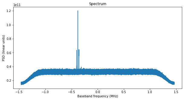
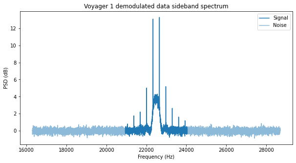
The first figure is the spectrum of the polyphase filterbank channel that we have extracted. The residual carrier of Voyager 1, as well as the data subcarrier can be seen well above the noise (note that the scale is in linear units of power).

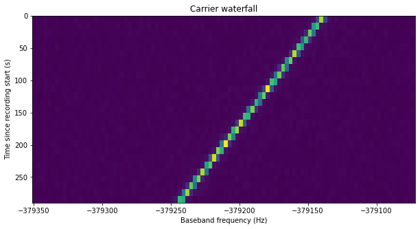
The next figure shows the waterfall of the carrier. The Doppler drift of the signal is apparent.

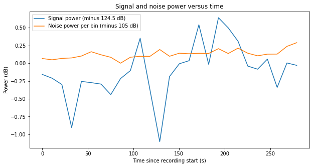
A measurement of the signal power of the residual carrier and the noise is done in order to estimate the C/N0 of the carrier. The measurement is done independently for each spectrum (time slice) in the waterfall. The bin where the carrier has maximum power is selected as centre and a few bins about this centre are used to measure the signal power (plus the noise in those bins). The noise power per bin is measured by averaging some 200 bins of noise to each side of the carrier (leaving some small guard band so as not to measure any power leaked from the carrier). The appropriate noise power is subtracted from the measurement of the signal power to obtain the signal power alone.

In the plot we see that there are large variations in the power of the carrier, of up to 1.5 dB. The SNR of the carrier will be measured later in a different way, confirming these variations.

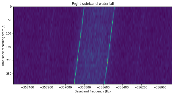
Finally, the next figure shows the waterfall of one of the sidebands. As we remarked in the previous post, the spectral lines are due to some long runs of zeros in the data, which is sent unscrambled. When these zeros pass through the convolutional encoder, an alternating 0101 sequence is produced due to the inverter in one of the branches of the encoder.

The power of each of the two sidebands is also measured in order to estimate the Eb/N0 that is present in the data modulation.

As expected, the three ON scans show the Voyager 1 signal, while the three OFF scans show only noise. The estimates of the C/N0 of the carrier and the Eb/N0 of the data subcarrier (adding up the power of both sidebands) are shown in the table below.

Scan	Carrier C/N0 (dB)	Data Eb/N0 (dB)
11	23.74	6.33
13	20.49	3.13
15	23.21	5.90

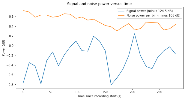
It is noteworthy that the middle ON scan has much worse SNR, approximately 3 dB less than the other scans. The figure below shows the signal and noise power measurement. The gain normalization is the same in all the recordings, so we see that the reduction of SNR is mainly due to an increase in the noise, which is around 3 dB stronger than in scan 11, and shows a large variation during the 5 minutes that the scan lasts. I do not know why the noise in this scan has increased so much.

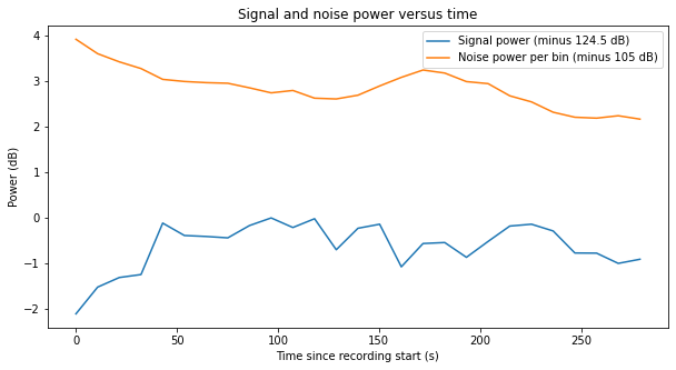
The last ON scan shows a behaviour that is similar to the first scan, although the SNR is some 0.5 dB worse. Again, there are large variations in the estimate of signal power.

The SNR of the middle ON scan (number 13) is in fact too low to decode the telemetry signal, so we will only use the first and last ON scans (numbers 11 and 15).

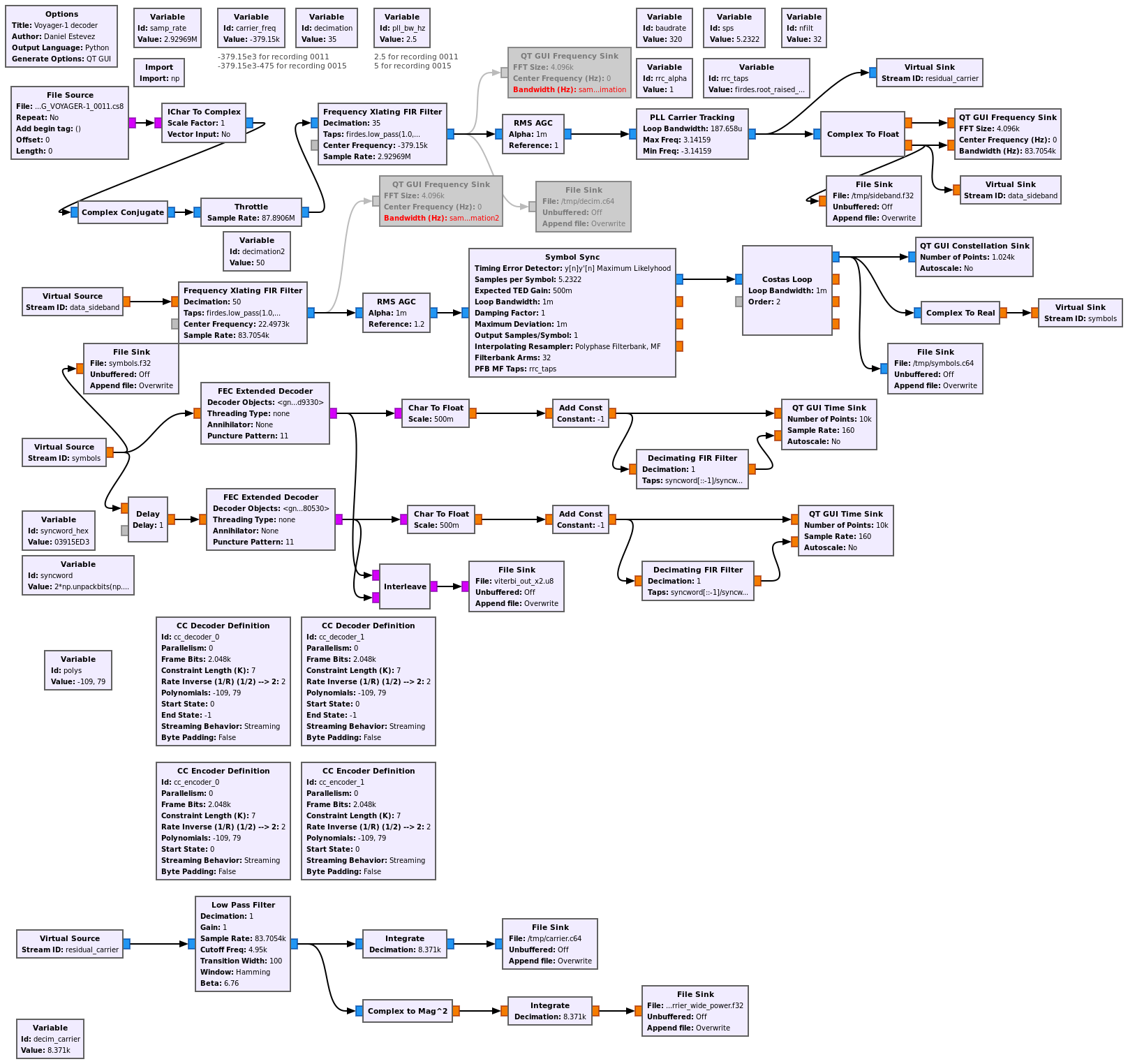
GNU Radio decoder

The GNU Radio decoder flowgraph is based on the flowgraph that I used in the previous post. It can be seen in the figure below (click on the figure to view it in full size). The flowgraph can be downloaded here.

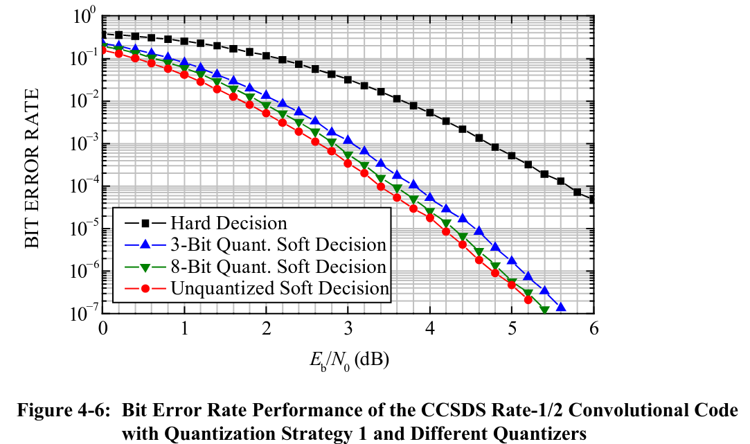
In comparison to the recording from 2015, which was easy to decode, these recordings are more difficult to decode, since the SNR is closer to the decoding threshold. The figure below, which is taken from the CCSDS TM Synchronization and Channel Coding Green Book, shows the BER of the rate 1/2 convolutional code used by Voyager 1. Frames are 7680 bits long, so for a FER of 1% we need a BER of \(10^{-6}\). This is achieved at 4.8 dB Eb/N0. We see that we have somewhat more than 1 dB of margin, so in principle things look good.

However, in practice the decoder doesn’t work so well. First, there’s always going to be some implementation losses in the decoder. Also, as we will see below, the large variations in signal power (of around 1 dB) that we have noticed above will give problems, causing burst errors in the Viterbi decoder output.

To try to understand the performance of the decoder better and see if it could be improved, I have tried to monitor the SNR of the data subcarrier in different points of the decoding chain. The GNU Radio flowgraph outputs to a File Sink in several intermediate steps. The signal is then analyzed in a Jupyter notebook to estimate its Eb/N0. These points are described in the sections below.

PLL output

The first intermediate step where the SNR is measured is the output of the PLL. Assuming an ideal carrier phase recovery, the two sidebands of the data subcarrier should add coherently, yielding the Eb/N0 that has been estimated above by adding the power of the two sidebands. However, the PLL does not track the carrier signal perfectly, so some power will be lost in the coherent combination of the data sidebands.

The calculations and plots are done in this Jupyter notebook. The figure below shows the data subcarrier at the output of the PLL. The FFT frequency resolution is 1.28 Hz. This makes visible not only the two tones due to the 010101 sequences in the symbols, but also their odd harmonics. These are caused by the square pulse shape filter.

In fact, the power decay of these harmonics matches that of a square wave, which is \(20 \log_{10} k\), so that the 3rd harmonic of a square wave is 9.54 dB below the fundamental, the 5th is 13.98 dB down, the 7th is 19.08 dB down, and the 11th is 20.83 dB down. We need to take into account that the PSD shows (S+N)/N rather than S/N. Assuming an (S+N)/N of the fundamental of 13 dB (which is more or less what we see in the plot), the (S+N)/N of the square wave odd harmonics would be 4.92, 2.45, 1.42 and 0.91 dB, which agrees with what we see here.

The area marked in dark blue in the plot is used to measure the signal plus noise power, and the area marked in light blue is used to measure the noise power. This gives the following Eb/N0 estimates for the data subcarrier after the PLL. The estimates done in the waterfall are shown for comparison.

Scan	PLL output Eb/N0 (dB)	Waterfall Eb/N0 (dB)	Loss (dB)
11	5.97	6.33	0.36
15	5.32	5.90	0.58

The cause of losses in the PLL are the phase errors in the carrier phase recovery. To put things in perspective, it is good to see what constant phase error would give the losses we observe. Since the loss in dB units is \(20 \log_{10}(cos \theta)\), where \(\theta\) is the phase error in radians, we see that a loss of 0.36 dB corresponds to a phase error of 16.4 degrees, and a loss of 0.58 dB corresponds to a phase error of 20.7 degrees.

The variance for the PLL phase error is approximately \(\sigma^2 = 1/\rho\), where \(\rho\) denotes the loop SNR, which can be computed as \(\rho = C/(N_0B_L)\), with \(B_L\) the loop bandwidth. More precisely, the PLL phase error distribution is a Tikhonov distribution with parameter \(\kappa = \rho\). For large \(\rho\), the Tikhonov distribution can be approximated by a normal distribution with variance \(1/\rho\). For more details about the PLL error, see for instance this paper. The corresponding carrier C/N0’s, loop bandwidths and phase error standard deviations are shown in this table.

Scan	Carrier C/N0 (dB)	Loop bandwidth (Hz)	Phase error \(\sigma\) (deg)
11	23.74	2.5	6.26
15	23.21	5	8.85

Note that a loop bandwidth of 5 Hz was used in scan 15 because the loop bandwidth of 2.5 Hz didn’t lock the loop properly.

These phase errors due to AWGN are significantly smaller than the phase errors of 16.4 and 20.7 degrees that we have mentioned above.

We can be more precise and compute the average power loss using the phase error Tikhonov distribution\[f(\theta) = \frac{\exp(\rho \cos \theta)}{2\pi I_0(\rho)}.\]Assuming that the subcarrier has power one at the input of the PLL, the average power of the subcarrier at the PLL output is\[\int_{-\pi}^\pi \cos^2(\theta) f(\theta)\, d\theta.\]This integral can be evaluated numerically for the values of \(\rho\) corresponding to each of the scans we are studying. We obtain losses of 0.05 dB and 0.10 dB for scans 11 and 15 respectively. These are much smaller than the losses we are observing.

Another source of error in PLLs is the steady state error due to higher order dynamics that are not modelled by the loop filter. For a loop filter of order 2, such as the one used by the PLL blocks in GNU Radio, the steady state error is\[\widetilde{\varphi}_{ss} \approx \frac{1}{2B_L^2}\varphi”.\]The exact value depends on the of the placement of the loop poles, but it is proportional to \(\varphi”/B_L^2\).

In our case, the Doppler drift rate is approximately 110 Hz over 300 seconds. This gives 2.3 rad/s². With a loop bandwidth of 2.5 Hz, we get a steady state error of 10.5 degrees, and with a loop bandwidth of 5 Hz we get a steady state error of 2.6 degrees. In the case of scan 11 this might account for the losses we see, since, roughly speaking, 11 degrees of steady state error plus 6 degrees of error due to noise would give the 17 degrees of error that correspond to the 0.36 dB loss we are seeing. In the case of scan 15 this doesn’t account for the losses, since we only have 3 degrees of steady state error plus 9 degrees of error due to noise, but we need a total of 21 degrees of error to explain the 0.58 dB loss.

It might be a good idea to remove the Doppler drift (which is almost a constant) to reduce the stress on the PLL and check if this reduces the PLL losses.

Something else that can be measured at the output of the PLL is the subcarrier frequency. By using the two strongest spectral lines, we can measure a frequency of 22497.3 Hz. This is an error of -117.9 ppm with respect to the nominal 22.5 kHz subcarrier. According to NASA HORIZONS, the range-rate at the time when the recording was made was 31.599 km/s. This would give a Doppler of -105.4 ppm, which agrees with the observed value. However, we need to take into account that the FFT resolution is not good enough to measure this accurately, as one FFT bin corresponds to 56.9 ppm of 22.5 kHz.

Costas loop output

The data subcarrier is processed with the Symbol Sync GNU Radio block to perform pulse shape filtering and symbol clock recovery. The maximum likelihood time error detector is used. This forces us to use a pulse shape with continuous derivate, since the maximum likelihood TED needs the derivative filter. Thus, instead of using a square pulse shape we use a root-raised cosine pulse shape. The excess bandwidth is set to 1.0, since that seems to work best regarding output SNR. The loop bandwidth is set to a low value. After symbol synchronization, a Costas loop is used to recover the residual subcarrier phase and frequency. It uses a low loop bandwidth.

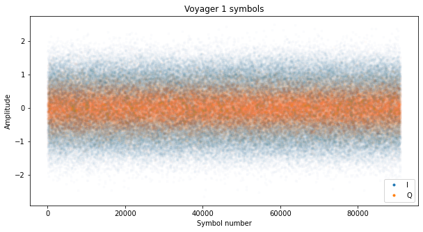
At the output of the Costas loop we should have the optimally sampled and filtered symbols in the I component, and noise in the Q component. The figure below shows the symbols obtained from scan 11. The first 5000 symbols have been thrown away, since the loops haven’t locked yet.

To estimate the SNR of the signal at this point we use the \(M_2M_4\) estimator described in the paper “A Comparison of SNR estimation techniques for the AWGN channel“. For a complex signal, this estimator is\[\frac{\sqrt{2M_2^2-M_4}}{M_2 – \sqrt{2M_2^2-M_4}},\]where \(M_2\) and \(M_4\) denote the second and fourth order moments respectively:\[M_2 = E[|x_n|^2],\quad M_4 = E[|x_n|^4].\]

In the table below we compare the results of this SNR estimator with the SNR estimates done before symbol synchronization.

Scan	Costas output Eb/N0 (dB)	PLL output Eb/N0 (dB)	Loss (dB)
11	5.40	5.97	0.57
15	4.77	5.32	0.55

Again, we have noticeable losses in this step of the decoder chain. Some of the losses can be explained by the mismatch between the transmit pulse shape filter (which is is a square shape) and the receiver filter (for which we are using an RRC filter). Here there is an opportunity for improvement by trying to use a square pulse shape in the receiver. Loop jitter can also explain some of the losses, but however the loop bandwidths are already set quite narrow to minimize jitter.

BCJR decoder

Usually, we would send the soft symbols to a Viterbi decoder, since Voyager 1 uses the typical CCSDS \(k=7, r=1/2\) convolutional code. However, the SNR is not good enough for error-free decode. When trying to study the contents of the frames to do reverse engineering, it can be rather hard to do so when there are bit errors, because some of the patterns we spot may be caused by bit errors rather than by the actual contents of the frames. It is much more helpful to have some soft output FEC decoder, since that gives us a level of confidence in the decoded data that we can use as a guide when interpreting the output.

Instead of using a soft output Viterbi algorithm, I have decided to use the BCJR algorithm. The whole output from each scan is processed at once by the BCJR decoder. The implementation of the decoder follows Algorithm 4.2 in the book “Iterative Error Correction” by Sarah Johnson. As in this book, the implementation I have done favours readability rather than efficiency. The BCJR decoder and the related plots are implemented in this Jupyter notebook.

To try to achieve the best performance with the BCJR decoder, we attempt to give it the best possible estimate on the noise variance \(\sigma^2\). To do so, we run the decoder with an initial estimate. We run hard decision on the BCJR output and encode the result with the convolutional code. We use this to wipe-off the data in our symbols. There are some symbol errors still, but most of the symbols are correct. Then we can measure the mean and variance of the wiped-off symbols, and use that to supply the BCJR decoder an improved estimate of \(\sigma^2\). We repeat this process a few times to improve the results.

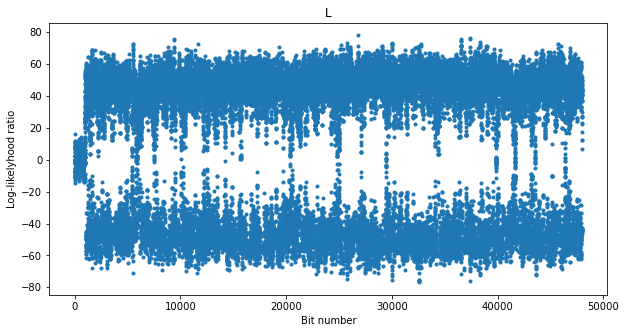
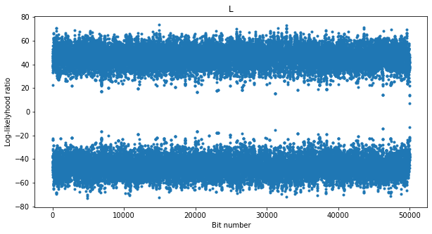
The figure below shows the soft output of the BCJR decoder, which is the log-likelihood ratio for the bits. At the beginning the output is around zero because the loops haven’t locked yet. Then we see that most of the time the decoder is able to correct all the errors, but there are several times when the log-likelihood ratio drops close to zero. As we will see later, these seem to correspond to drops in the CN0 of the carrier.

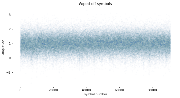
The next figure shows the wiped-off symbols, using the re-encoded hard decision on the output from the BCJR decoder. We see that most of the symbols have been wiped off correctly. This is used to estimate the amplitude and noise variance of the signal.

We can use the amplitude and noise variance of this wiped-off signal to estimate the Eb/N0. If we denote by \(y_n\) the wiped-off symbols, an estimate of the SNR is given by \(E[y_n]/(2E[|y_n|^2])\). Alternatively, we can use equation (31) in the paper “A Comparison of SNR estimation techniques for the AWGN channel“, which is known as the SNV TxDA estimate for a real signal. This gives a very similar result.

The table below compares the results of this estimate with the \(M_2M_4\) estimate obtained at the output of the Costas loop. We see that the results are slightly lower. Perhaps the reason is due to the occasional symbol errors after wipe-off, or just to the different estimators used

Scan	Wipe-off Eb/N0 (dB)	Costas output Eb/N0 (dB)	Difference (dB)
11	5.26	5.40	0.14
15	4.61	4.77	0.16

To assess the performance of the BCJR decoder at this SNR, we can build a simulated signal on AWGN and run it through the decoder. These are the results of decoding a simulated signal at the same SNR as scan 11. We see that the decoder works very well, and there should be no errors at its output. This matches the fact that a convolutionally encoded signal can be decoded without problems at an Eb/N0 of 5 dB.

Therefore, we see that the problem with our recordings is that the SNR is not stationary. There are some sudden SNR drops that cause errors in the BCJR decoder (or in the Viterbi decoder).

Carrier SNR

These SNR drops might be caused by several factors. The most obvious cause are drops in the SNR of the phase-modulated signal. There are other possible explanations, such as instability in the phase/clock of the signal, which would cause larger errors in the loops.

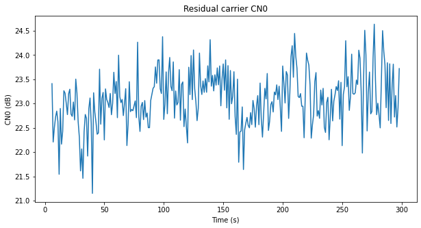
To try to understand the cause of these drops, we perform an SNR estimate on the residual carrier. We have already such an estimate using the waterfall, but the time resolution was not high enough to see the drops clearly.

To perform the SNR estimate, we take the output of the PLL and run it through a low pass filter with a noise bandwidth of 10 kHz. The output of this filter is integrated coherently down to a 10 Hz rate. Additionally, the complex magnitude squared of the filter output is taken and integrated down to a 10 Hz rate. These two outputs are processed in a Jupyter notebook.

The next figure shows the 10 Hz coherent integrations of the PLL output corresponding to scan 11. As expected, the residual carrier appears in the I component, while the Q component contains noise and leakage from the carrier due to phase noise. In fact we see that the noise variance in the Q component is much larger than in the I component, so the extra noise variance must be due to phase noise (see above for some notes on the PLL phase jitter).

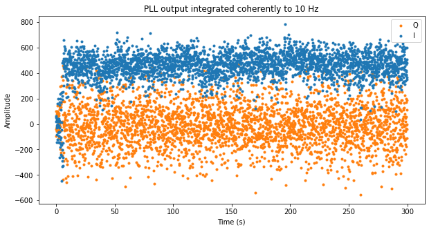
We also see some sudden drops in the amplitude of the I component. There is an AGC in the flowgraph, but since the AGC acts on the full 83.7 kHz bandwidth, the noise power dominates the AGC input, so the changes in amplitude we see here correspond to changes in SNR (which actually are caused by changes in the signal power).

The plot below shows an estimate of the CN0 of the residual carrier with a resolution of one second. This has been obtained by averaging the 10 Hz measurements in groups of 10 and then noting that the coherent integrations measure signal power plus noise in 10 Hz, while the power at the filter output measures signal power plus noise in 10 kHz.

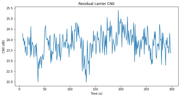
The changes in the CN0 show the same behaviour as in the plot with lower temporal resolution obtained from the waterfall. The CN0 has large variations of up to 2.5 dB. It seems that the drops in the log-likelihood ratio of the BCJR are somewhat related to these drops in CN0, but the match is not completely perfect.

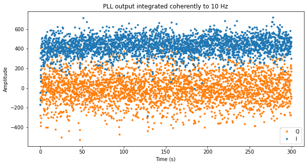
The two figures below show the corresponding plots for scan 15.

Telemetry frames

We can take the log-likelihood ratios produced by the BCJR decoder and detect the ASM, which is 0x03915ED3, in order to correct the for the possible 180º phase ambiguity in the Costas loop and to align with the telemetry frames. Then we can do a raster plot of the log-likelihoods of the bits in each of the frames.

The raster plot is done by sections of 128 bits. In the raster plots each of the frames is shown as a row, while each column corresponds to the bit position in the frame. The red colours correspond to ones (positive log-likelihood ratios), and the blue colours corresponds to zeros (negative log-likelihood rations). Lighter colours correspond to log-likelyhood ratios with smaller magnitude, which mean that the BCJR decoder is not so sure about the correct output. The first plot is shown below.

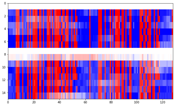
First we can see the 32 bit ASM. Then we see an interesting pattern around bit 40 that changes every other frame. Around frame 50 we see a counter which is at least 6 bits wide. After the first 64 bits we have almost a repetition of the same data. The same 32 bit ASM appears on position 64, we have the changing pattern around bit 105, and also the counter around bit 115. We note that some of the bits with a lighter colour have decoding errors, but the log-likelihood information from the BCJR decoder helps us spot and discard these.

The Voyager 1 frames are 7680 bits long, so there are a total of 60 plots of segments of 128 bits. All these are shown in this Jupyter notebook. Other than finding a few binary counters and observing the general structure of the frames, I haven’t been able to figure out the meaning of any of this data.

Data and results

Most of the data used in this post (excepting large files), as well as the code used for the calculations and figures can be found in this repository.